Generate the shape coefficient (Ce)

The shape coefficient is the area-weighted mean of Cp over each zone of the body. Zones come from a 3D box grid; every triangle is assigned to a zone by its centroid. The v3 pipeline attaches the mesh, builds a zoning_grouping, then aggregates Cp per zone with an area_weighted_mean.

Set up a working directory

A pipeline template declares its inputs, ops and outputs with paths that are resolved relative to the template file. The shipped example templates live under fixtures/tests/pressure/templates/ and reference sibling ../data/ and ../galpao/ folders, so we copy the templates and the fixture data into a single scratch directory and run from there. In a real project you would instead point the template at your own data and run cfdmod run <template>.yaml directly.

%matplotlib inline
import pathlib
import shutil
import tempfile


def find_fixtures() -> pathlib.Path:
    """Walk up from the current directory to locate the repo fixtures."""
    for base in [pathlib.Path.cwd(), *pathlib.Path.cwd().parents]:
        candidate = base / "fixtures" / "tests" / "pressure"
        if candidate.is_dir():
            return candidate
    raise FileNotFoundError("could not locate fixtures/tests/pressure")


fixtures = find_fixtures()
workdir = pathlib.Path(tempfile.mkdtemp(prefix="cfdmod_pressure_"))
for name in ("data", "galpao", "templates"):
    shutil.copytree(fixtures / name, workdir / name)
(workdir / "out").mkdir(exist_ok=True)

print("working directory:", workdir)

working directory: /tmp/cfdmod_pressure_cxeevg4i

Compute Cp first

The force, moment and shape coefficients all consume a Cp time series. We run the cp.yaml template first; it writes ./out/cp.time_series inside the working directory, which the template below reads back in.

from cfdmod import load_template, run_template
from cfdmod.adapters.xdmf_h5 import XdmfH5Storage

storage = XdmfH5Storage(pathlib.Path("/"))
run_template(load_template(workdir / "templates" / "cp.yaml"), storage=storage)
print("Cp time series written to", workdir / "out")

Cp time series written to /tmp/cfdmod_pressure_cxeevg4i/out

The Ce pipeline template

zoning_grouping partitions the mesh into a x_intervals x y_intervals x z_intervals box grid; field_series_for_groups with agg: area_weighted_mean then collapses Cp to one series per zone.

print((workdir / "templates" / "ce.yaml").read_text())

# Ce pipeline template (v3 schema).
#
# Per-zone shape coefficient via area-weighted-mean of Cp. Zones come
# from a 3D box grid (x_intervals x y_intervals x z_intervals);
# triangles are assigned by centroid.
name: ce_default

inputs:
  cp:
    kind: surface
    path: ./out/cp.time_series

pipeline:
  - id: cp_with_mesh
    kind: mesh_attach
    source: cp
    mesh: ../galpao/galpao.normalized.lnas

  - id: cp_zoned
    kind: zoning_grouping
    source: cp_with_mesh
    mesh: ../galpao/galpao.normalized.lnas
    x_intervals: [0.0, 125.0, 250.0]
    y_intervals: [0.0, 80.0, 170.0]
    z_intervals: [0.0, 10.0, 20.0]

  - id: ce
    kind: field_series_for_groups
    source: cp_zoned
    grouping: zone
    field: cp
    agg: area_weighted_mean
    out: ce

outputs:
  ce: {source: ce, path: ./out/ce.time_series}

Run the pipeline

bindings = run_template(load_template(workdir / "templates" / "ce.yaml"), storage=storage)
sorted(bindings)

[2026-07-06 01:03:07,594] [INFO] - cfdmod - apply_groupings: 1 grouping(s) on mesh with 2915 triangle(s) and 20 surface(s)
[2026-07-06 01:03:07,597] [INFO] - cfdmod -   [0] ByZoningGrouping produced 8 group(s): ['0-0-0', '0-0-1', '0-1-0', '0-1-1', '1-0-0']...

['ce', 'cp', 'cp_with_mesh', 'cp_zoned']

Per-zone shape coefficient

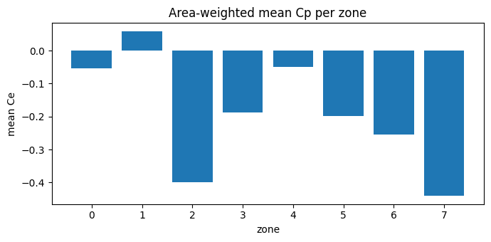
ce is a GroupsDataSource with one row per occupied zone. We show the time-averaged Ce per zone.

import pandas as pd

from cfdmod.core.grouping import groups_in

ce = bindings["ce"]
pg = ce.parent_grouping
labels = [pg.label(g) for g in groups_in(pg)]
series = ce.fields.read("ce")
df = pd.DataFrame({"ce_mean": series.mean(axis=1)}, index=labels)
df.index.name = "zone"
df

	ce_mean
zone
0	-0.054599
1	0.058763
2	-0.399228
3	-0.187045
4	-0.048913
5	-0.198927
6	-0.254235
7	-0.440501

import matplotlib.pyplot as plt

fig, ax = plt.subplots(figsize=(7, 3.5))
ax.bar(df.index, df["ce_mean"])
ax.set_xlabel("zone")
ax.set_ylabel("mean Ce")
ax.set_title("Area-weighted mean Cp per zone")
plt.tight_layout()
plt.show()