Moment Coefficient
The Moment Coefficient, \(C_M\), is a dimensionless parameter that provides a generalized representation of the resultant moment experienced by an object within a fluid flow. It offers a means to evaluate the cumulative effect of pressure coefficients, \(c_p\) across different regions of an object’s surface and how these pressures translate into aerodynamic moment forces.
\(C_M\) is a fundamental tool for torsional effects for the design and analysis of aerodynamic components.
Definition
Similarly to the force coefficient, this coefficient is defined as a resulting moment coefficient of a body.
It is defined as a sum of the resulting moment for each triangle of each surface of the body:
The position vector \(r_o\) is defined for each triangle, from a common arbitrary points \(o\). One can also define it for each axis direction:
We define the nominal volume ($V_{nom}$) as a user input. This is done to let the user define how they want to calculate its value. For example, considering a rectangular tall building:
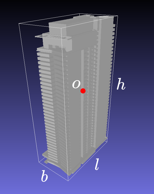
The nominal volume could be calculated with:
Use Case
A common application of the moment coefficient requires sectioning the body in different sub-bodies. To do so, the same logic applied to the force coefficient is used to determine the respective sub-body of each of the body’s triangles. If its center lies inside the sub-body volume, then it belongs to it.
The result is a sectionated body in different sub-bodies for each interval. When sectioning the body, the respective nominal volume should be the same as the sub-body nominal volume.
Note
Check out the definitions section for more information about surface, body and sub-body definitions.
Like the other coefficients, we can apply statistical analysis to the moment coefficient.
By definition, the moment coefficient is a property of a body.
It is used for primary and secondary structures design, such as canopies. It can also be used for evaluating the resultant wind torsional effect over a building or the building paviments. It can be seen as the resulting torsion effect of the wind induced stress over a body.
Lever-origin strategies
The moment center per region is configured on
cfdmod.MomentBodyConfig. v2 supports three strategies:
lever_strategy="fixed"(default) – every triangle uses the body’slever_origintuple.lever_strategy="region_base"– per region, the moment center is derived from the region’s triangle vertices as \((\overline{x}, \overline{y}, \min z)\). This matches the footprint centroid at the lowest z and is the natural choice for overturning moments about the base of each container.lever_strategy="region_bbox_corners_xy"– expand the body into four independent runs (xmin_ymin,xmin_ymax,xmax_ymin,xmax_ymax); each run lands as its ownCm.{cfg_lbl}.{body}.{case}.time_series.{h5,xdmf}plus its ownstats.h5subgroup. Useful for a worst-case overturning-moment scan around the footprint.
For HFPI-style analyses where the center of mass per region is known
externally, set region_lever_origins={region_int: (x, y, z), ...} –
that overrides the strategy on those regions only. To scan an arbitrary
labelled set of candidate centers, use
lever_origin_cases={"label": {region_int: (x, y, z), ...}, ...};
each case becomes an independent run with the same naming convention as
region_bbox_corners_xy.
Artifacts
The user provides:
Cp timeseries XDMF+H5 produced by
run_cp.Parameters (
CmCaseConfig): bodies, sub-body zoning, and the lever-origin spec described above. Pass either a YAML path or an in-memory instance.Mesh (optional):
.lnas/.stl/.h5/.xdmf. Only the LNAS variant carries authored surfaces; the others present the mesh as a single"all"surface. When omitted, the geometry comes from the cp timeseries H5.
Outputs (flat under output):
Cm.{cfg_lbl}.{body}[.{case}].time_series.{h5,xdmf}– one file per body (or per case, when a multi-case strategy is in use). Each file embeds the body’s mesh and carriescm_x/cm_y/cm_zgroups – pick the direction from the ParaView Attribute selector on the same animation.stats.h5/stats.xdmf– combined statistics; Cm lands under/cm_{x,y,z}/{cfg_lbl}/{body}[.{case}]/with the body’s mesh embedded so the<Grid>references topology of matching length.Each output H5 carries the post-processing config under
/processing_metadata/.
Usage
Reference parameters file:
bodies:
  marquise:
    surfaces: [list_of_surfaces_of_marquise]
  lanternim:
    surfaces: [list_of_surfaces_of_lanternim]
  building:
    surfaces: [building]
moment_coefficient:
  measurement_1:
    bodies:
      - name: marquise
        lever_origin: [0, 10, 10]
    directions: ["x", "y", "z"]
    # Nominal volume to use for calculations
    nominal_volume: 10
    statistics:
      - stats: "mean"
      - stats: "rms"
      - stats: "skewness"
      - stats: "kurtosis"
      - stats: "min"
        params:
          method_type: "Absolute"
      - stats: "max"
        params:
          method_type: "Absolute"
    # Apply transformations before indexing the regions
    transformation:
      translation: [0, 0, 0]
      rotation: [0, 0, 0]
      fixed_point: [0, 0, 0]
  measurement_2:
    bodies:
      - name: building
        lever_origin: [0, 10, 10]
        sub_bodies: # Optional, default is the whole body
          z_intervals: [0, 10, 20]
    directions: ["x", "y", "z"]
    # Nominal volume to use for calculations
    nominal_volume: 10
    statistics:
      - stats: "mean"
      - stats: "rms"
      - stats: "skewness"
      - stats: "kurtosis"
      - stats: "min"
        params:
          method_type: "Absolute"
      - stats: "max"
        params:
          method_type: "Absolute"
    # Apply transformations before indexing the regions
    transformation:
      translation: [0, 0, 0]
      rotation: [0, 0, 0]
      fixed_point: [0, 0, 0]
From Python:
from cfdmod import run_cm, CmCaseConfig
run_cm(
    cp_h5="output/cp.default.time_series.h5",
    cfg_path=CmCaseConfig.from_file("cm.yaml"),
    output="output",
    # mesh_path optional; omitting it reads geometry from the cp H5
)
CLI:
python -m cfdmod pressure cm \
   --cp     {CP_TIMESERIES_H5} \
   --config {CONFIG_PATH} \
   --output {OUTPUT_PATH}
The Sphinx-bundled calculate_Cm.ipynb notebook
covers a single body with a fixed lever origin; for the multi-region
region_bbox_corners_xy scan and per-container overturning moments,
see notebooks/process_container_pack.ipynb in the repository root.
Data format
Note
The rule for determining the region_idx is based on the region index and the body name. Input mesh can have multiple bodies, and each of them can be applied a specific zoning/region rule. Because of that, region_idx has to be composed by the zoning region index joined by “-” and the body name. This also guarantee that even if different bodies lie on the same region, the interpreted region for each of them will be different
Note
For more information about the normalized time scale (\(t^*\)), check the Normalization section
time_idx/region_idx |
Normalized time (\(t^*\)) |
0-Body1 |
1-Body1 |
0-Body2 |
|---|---|---|---|---|
0 |
10000 |
1.25 |
1.15 |
-1.1 |
1 |
11000 |
1.5 |
0.9 |
-1.15 |
time_idx/region_idx |
Normalized time (\(t^*\)) |
0-Body1 |
1-Body1 |
0-Body2 |
|---|---|---|---|---|
0 |
10000 |
1.25 |
1.15 |
-1.1 |
1 |
11000 |
1.5 |
0.9 |
-1.15 |
time_idx/region_idx |
Normalized time (\(t^*\)) |
0-Body1 |
1-Body1 |
0-Body2 |
|---|---|---|---|---|
0 |
10000 |
1.25 |
1.15 |
-1.1 |
1 |
11000 |
1.5 |
0.9 |
-1.15 |
region_idx |
max |
min |
mean |
std |
skewness |
kurtosis |
|---|---|---|---|---|---|---|
0-Body1 |
1.25 |
0.9 |
1.1 |
0.2 |
0.1 |
0.15 |
1-Body1 |
1.15 |
0.95 |
1.13 |
0.19 |
0.11 |
0.13 |
region_idx |
max |
min |
mean |
std |
skewness |
kurtosis |
|---|---|---|---|---|---|---|
0-Body1 |
1.25 |
0.9 |
1.1 |
0.2 |
0.1 |
0.15 |
1-Body1 |
1.15 |
0.95 |
1.13 |
0.19 |
0.11 |
0.13 |
region_idx |
max |
min |
mean |
std |
skewness |
kurtosis |
|---|---|---|---|---|---|---|
0-Body1 |
1.25 |
0.9 |
1.1 |
0.2 |
0.1 |
0.15 |
1-Body1 |
1.15 |
0.95 |
1.13 |
0.19 |
0.11 |
0.13 |
region_idx |
point_idx |
|---|---|
0-Body1 |
0 |
1-Body1 |
1 |
region_idx |
x_min |
x_max |
y_min |
y_max |
z_min |
z_max |
Lx |
Ly |
Lz |
|---|---|---|---|---|---|---|---|---|---|
0-Body1 |
0 |
100 |
0 |
50 |
0 |
20 |
0.5 |
0.8 |
0.1 |
1-Body1 |
100 |
200 |
0 |
50 |
0 |
20 |
0.5 |
0.8 |
0.1 |