Generate the pressure coefficient (Cp)

The pressure coefficient normalizes the surface pressure by the free-stream dynamic pressure:

\[C_p(t) = \frac{p(t) - p_{\infty}(t)}{q}, \qquad q = \tfrac{1}{2}\, \bar{\rho}_{\infty}\, U_H^2 .\]

In cfdmod v3 this is expressed as a pipeline template: a small YAML document listing the inputs (body pressure, static-pressure probe), a sequence of composable ops, and the outputs. This notebook runs the shipped cp.yaml template against the galpao wind-tunnel fixture.

Set up a working directory

A pipeline template declares its inputs, ops and outputs with paths that are resolved relative to the template file. The shipped example templates live under fixtures/tests/pressure/templates/ and reference sibling ../data/ and ../galpao/ folders, so we copy the templates and the fixture data into a single scratch directory and run from there. In a real project you would instead point the template at your own data and run cfdmod run <template>.yaml directly.

%matplotlib inline
import pathlib
import shutil
import tempfile


def find_fixtures() -> pathlib.Path:
    """Walk up from the current directory to locate the repo fixtures."""
    for base in [pathlib.Path.cwd(), *pathlib.Path.cwd().parents]:
        candidate = base / "fixtures" / "tests" / "pressure"
        if candidate.is_dir():
            return candidate
    raise FileNotFoundError("could not locate fixtures/tests/pressure")


fixtures = find_fixtures()
workdir = pathlib.Path(tempfile.mkdtemp(prefix="cfdmod_pressure_"))
for name in ("data", "galpao", "templates"):
    shutil.copytree(fixtures / name, workdir / name)
(workdir / "out").mkdir(exist_ok=True)

print("working directory:", workdir)

working directory: /tmp/cfdmod_pressure_u6sirp_9

The Cp pipeline template

The template subtracts the static reference pressure per timestep (sub), divides by the dynamic pressure via a constant scale factor (1 / q), and finally reduces the time axis to per-element statistics (mean / rms / min / max).

print((workdir / "templates" / "cp.yaml").read_text())

# Cp pipeline template (v3 schema).
#
# Reads body pressure and a static-pressure probe from disk, computes
# Cp = (p - p_ref) / dyn_pressure, optionally rescales time, and writes
# the time-resolved Cp series plus mean/rms/peak statistics.
#
# Anything you'd previously have configured under
# pressure_coefficient.default.statistics in cp_params.yaml now lives
# under the `statistics` step. Everything else is pipeline composition.
name: cp_default

inputs:
  body:
    kind: surface
    path: ../data/bodies.galpao
  p_ref:
    kind: points
    path: ../data/points.static_pressure

pipeline:
  # 1. Subtract the static reference per timestep (column-wise broadcast,
  #    rule 2). The result lives on a new "cp" field on the body source.
  - id: cp_unscaled
    kind: sub
    source: body
    rhs: p_ref
    field: pressure
    out: cp

  # 2. Divide by dynamic pressure. q_inf = 0.5 * rho * U_H^2
  #    Here U_H = 0.05, rho = 1.0 -> q = 0.00125. Scale = 1 / q.
  - id: cp_t
    kind: scale
    source: cp_unscaled
    field: cp
    factor: 800.0

  # 3. Per-element statistics over the full time axis.
  - id: cp_stats
    kind: statistics
    source: cp_t
    field: cp
    kinds: [mean, rms, min, max]

outputs:
  cp_timeseries:
    source: cp_t
    path: ./out/cp.time_series
  cp_stats:
    source: cp_stats
    path: ./out/cp.stats

Run the pipeline

The runner is backend-agnostic. Here we use XdmfH5Storage, which reads and writes the on-disk XDMF+H5 layout; notebooks and tests can instead use the in-memory MemoryStorage with the exact same recipe code. run_template returns a dict mapping every step id (and input) to its DataSource.

from cfdmod import load_template, run_template
from cfdmod.adapters.xdmf_h5 import XdmfH5Storage

storage = XdmfH5Storage(pathlib.Path("/"))
bindings = run_template(load_template(workdir / "templates" / "cp.yaml"), storage=storage)
sorted(bindings)

['body', 'cp_stats', 'cp_t', 'cp_unscaled', 'p_ref']

Inspect the time-resolved Cp

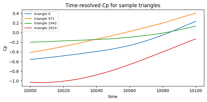
cp_t is a SurfaceDataSource with one row per mesh triangle and one column per timestep. We plot the Cp history of a handful of triangles.

import matplotlib.pyplot as plt
import numpy as np

cp_t = bindings["cp_t"]
times = cp_t.time.times()
cp = cp_t.fields.read("cp")
print("elements x timesteps:", cp.shape)

fig, ax = plt.subplots(figsize=(7, 3.5))
for idx in np.linspace(0, cp.shape[0] - 1, 4, dtype=int):
    ax.plot(times, cp[idx], label=f"triangle {idx}")
ax.set_xlabel("time")
ax.set_ylabel("Cp")
ax.set_title("Time-resolved Cp for sample triangles")
ax.legend(loc="best", fontsize=8)
plt.tight_layout()
plt.show()

elements x timesteps: (2915, 101)

Per-element statistics

The cp_stats output collapses the time axis to one value per triangle for each requested statistic.

import pandas as pd

stats = bindings["cp_stats"]
df = pd.DataFrame({name: stats.fields.read(name) for name in stats.field_names})
df.describe()

	mean	rms	min	max
count	2915.000000	2915.000000	2915.000000	2915.000000
mean	-0.203118	0.153959	-0.396791	0.106785
std	0.273381	0.062831	0.294066	0.250219
min	-0.949901	0.002697	-1.173019	-0.664139
25%	-0.390826	0.110966	-0.592470	-0.017977
50%	-0.212155	0.167677	-0.408554	0.130272
75%	-0.005807	0.203829	-0.187683	0.280762
max	0.455437	0.307976	0.339985	0.757790