Shape Coefficient¶

Shape coefficient describes the behavior of the resulting pressure applied to a surface. It can be interepreted as a resulting pressure coefficient inside a given region.

It allows us to assess how the local pressure at different points inside a region combine themselves.

Definition¶

The shape coefficient is a dimensionless form of the resulting pressure signal.

Consider a rectangular surface composed by triangles. At each of its triangles’ center, pressure signals are obtained. However, we can calculate the resulting force by summing the pressure load of each triangle. To do so, pressure is transformed into a force by multiplying by the respective triangle area.

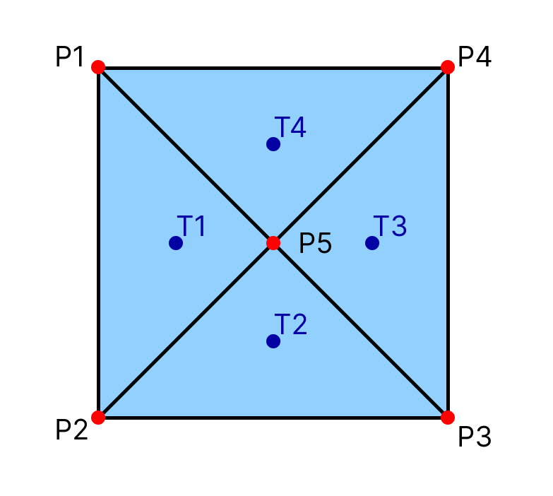
We can define a resulting force for each triangle as:

\[f_{i} = p_{i} A_{i} = c_{pi} q A_{i}\]

Even so, we can define a resulting force for the surface, by summing its triangles forces:

\[F_{res} = \sum{f_{i}} = p_{1} A_{1} + p_{2} A_{2} + p_{3} A_{3} + p_{4} A_{4} = q (c_{p1} A_{1} + c_{p2} A_{2} + c_{p3} A_{3} + c_{p4} A_{4})\]

Important

Some peaks (minimum or maximum) of the pressure coefficient signal can be cancelled when calculating the shape coefficient.

The shape coefficient is based on the definition of an area of influence. This area is delimited by x, y and z intervals. Each combination of the intervals results in a region.

Note

Check out the concepts section for more information about region and surface definitions.

To calculate the shape coefficient of a given region, the surface triangles which center lies inside this region must be filtered. Then, the resulting force is evaluated for the filtered triangles data. After that, the shape coefficient can be calculated. For the previous example, considering a case where only one region exists:

\[C_{e} = \frac{F_{res}}{q A_{region}} = \frac{(c_{p1} A_{1} + c_{p2} A_{2} + c_{p3} A_{3} + c_{p4} A_{4})}{A_{region}}\]

And we can obatin its maximum, minimum, RMS and average values.

Use Case¶

By definition, the shape coefficient is a property of a surface or an area. It is used to evaluate wind loads on primary and secondary structures, such as beans, coating and sealing components.

Structural engineers might use the shape coefficient for wind load evaluation on superficial and long elements.

For smaller components, it is essential to define small intervals for the region definition, which size should be comparable to the component of interest size.

For example, to evaluate the effect of wind pressure on windows, the intervals used for defining the shape coefficient regions should be about the window size, in a way that all triangles that form the window lie inside of this region.

It can also be used to evaluate the resulting wind effect over coating elements, mounted on roofs or walls, such as panels. Or even to evaluate the resulting effect over doors, and calculate the stress over its hinges.

Artifacts¶

The user provides:

Cp timeseries XDMF+H5 produced by run_cp.
Parameters (CeCaseConfig): zoning intervals, surface set/exclude/exception lists and statistics. Pass either a YAML path or an in-memory instance.
Mesh (optional): .lnas / .stl / .h5 / .xdmf. Ce slices triangles along the zoning planes and so produces a different output mesh than the input – the cut regions mesh.

Outputs (flat under output):

Ce.{cfg_lbl}.regions.stl – the cut regions mesh as STL for ParaView / QC use.
Ce.{cfg_lbl}.time_series.{h5,xdmf} – per-cut-triangle Ce timeseries on the cut mesh (root /Triangles + /Geometry is the cut mesh; per-timestep arrays under /ce/t{T}).
stats.h5 / stats.xdmf – Ce stats land under /ce/{cfg_lbl}/ with the cut mesh embedded so ParaView renders on the right topology.
Each output H5 carries the post-processing config under /processing_metadata/.

Usage¶

Reference parameters file:

shape_coefficient:
  pattern_1:
    zoning:
      # Relative path to this file
      yaml: "./zoning_params.yaml"
    statistics:
      - stats: "mean"
      - stats: "rms"
      - stats: "skewness"
      - stats: "kurtosis"
      - stats: "mean_eq"
        params:
          scale_factor: 0.61
      - stats: "min"
        params:
          method_type: "Peak"
          peak_factor: 3
      - stats: "max"
        params:
          method_type: "Absolute"
    # Apply transformations before indexing the regions
    transformation:
      translation: [0, 0, 0]
      rotation: [0, 0, 0]
      fixed_point: [0, 0, 0]

zoning_params.yaml¶

# Define a default region rule
global_zoning:
  x_intervals: []
  y_intervals: []
  z_intervals: []
# Optional
no_zoning: [] # Select the surfaces to ignore region mesh generation
# Optional
exclude: [] # Select surfaces to ignore when calculating shape coefficient
# Optional
exceptions:
  # Define a specific region rules
  zoning1:
    x_intervals: []
    y_intervals: []
    z_intervals: []
    surfaces: [] # Surface to overload the default rule

From Python:

from cfdmod import run_ce, CeCaseConfig
run_ce(
    cp_h5="output/cp.default.time_series.h5",
    cfg_path=CeCaseConfig.from_file("ce.yaml"),
    output="output",
    # mesh_path optional; omitting it reads geometry from the cp H5
)

CLI:

python -m cfdmod pressure ce \
   --cp     {CP_TIMESERIES_H5} \
   --config {CONFIG_PATH} \
   --output {OUTPUT_PATH}

The Sphinx-bundled calculate_Ce.ipynb notebook covers the full Ce workflow.

Data format¶

Important

All tables for shape coefficient listed below are defined for each of the body’s surfaces, unlike the other coefficients. The idea is to keep the processing for a single surface and not account for unrelated data.

Note

The rule for determining the region_idx is based on the region index and the surface name. Input mesh can have multiple surfaces, and each of them can be applied a specific zoning/region rule. Because of that, region_idx has to be composed by the zoning region index joined by “-” and the surface name. This also guarantee that even if different surfaces lie on the same region, the interpreted region for each of them will be different

Note

For more information about the normalized time scale (\(t^*\)), check the Normalization section

\(C_e(t)\)¶
time_idx/region_idx	Normalized time (\(t^*\))	0-Surface 1	1-Surface 1
0	0.0	0.25	0.35
1	1.0	0.23	0.32

\(C_e (stats)\)¶
region_idx	max	min	mean	std	skewness	kurtosis
0-Surface 1	1.25	0.9	1.1	0.2	0.1	0.15
1-Surface 1	1.15	0.95	1.13	0.19	0.11	0.13

\(Regions(indexing)\)¶
region_idx	point_idx
0-Surface 1	0
1-Surface 1	1

\(Regions(definition)\)¶
region_idx	x_min	x_max	y_min	y_max	z_min	z_max
0-Surface 1	0	100	0	50	0	20
1-Surface 1	100	200	0	50	0	20