Pressure Coefficient¶

The Pressure Coefficient, \(c_p\), is a dimensionless quantity that provides a generalized representation of the pressure distribution on a surface, or body, exposed to a fluid flow. It allows us to assess how the local pressure at a specific point differs from the surrounding free-stream pressure, accounting for the dynamic pressure of the fluid flow.

Definition¶

The pressure coefficient is a dimensionless form of the pressure signal. It is obtained by the following expression:

\[c_{p}(t) = \frac{p(t) - p_{\infty}(t)}{q}\]

By definition, the pressure coefficient is a local property for each triangle of the mesh.

Use Case¶

It is used primarily for analysis and interpretation of the measured data.

It should always be generated, since it is the first analysis step. It is a fundamental property of the pressure normalization, and it is used to calculate the other coefficients. However, it is not the final result to be delivered to clients.

Artifacts¶

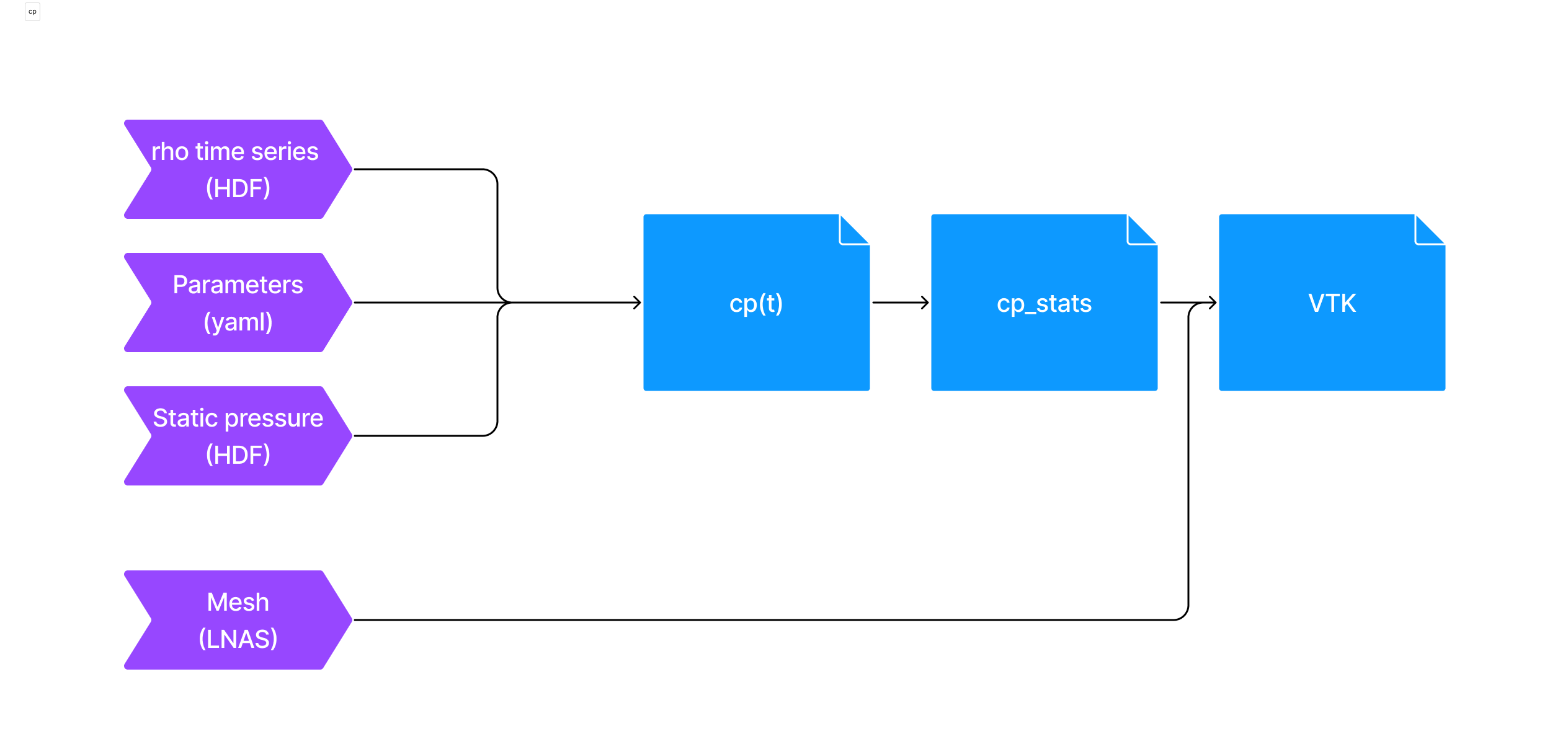
In order to use the pressure normalization module, the user has to provide a set of artifacts:

A lnas file: It contains the information about the mesh.
HDF time series: It contains the pressure signals indexed by each of the mesh triangles.
Parameters file: It contains the values for adimensionalization as well as other configs parameters.
Static reference pressure time series: It contains the pressure signals for probes far away from the building.

Which outputs the following data:

Dimensionless time series: pressure coefficient time series for each triangle.
Statistical results: statistical values for the pressure coefficient time series, for each triangle.
VTK File: contains the statistical values inside a mesh representation (VTK).

An illustration of the pressure coefficient module pipeline can be seen below:

Usage¶

The parameter file for converting the pressure data into pressure coefficient looks as follows:

pressure_coefficient:
  default:
    # Define how many chunks the output time series will be split into. Optional, defaults to 1
    number_of_chunks: 10
    # Select the time interval to filter the signal and calculate statistics
    timestep_range: [10000, 20000]
    # Velocity at the building interest height
    simul_U_H: 0.05
    # Simulation characteristic length scale for time scale conversion
    simul_characteristic_length: 0.8445
    # Define which statistics will be calculated
    statistics:
      - stats: "mean"
      - stats: "rms"
      - stats: "skewness"
      - stats: "kurtosis"
      - stats: "mean_eq"
        params:
          scale_factor: 0.61
      - stats: "min"
        params:
          method_type: "Absolute"
      - stats: "max"
        params:
          method_type: "Gumbel"
          peak_duration: 3 # in seconds
          event_duration: 600 # in seconds. Period of extreme event
          n_subdivisions: 10 # Number of subdivisions
          non_exceedance_probability: 0.78 # Confidence parameter in %
          full_scale_U_H: 40
          full_scale_characteristic_length: 22.4
      - stats: "max"
        params:
          method_type: "Peak"
          peak_factor: 3 # xtr = avg +- factor * rms
      - stats: "max"
        params:
          method_type: "Moving Average"
          window_size_interval: 3 # s
          full_scale_U_H: 40
          full_scale_characteristic_length: 22.4

To invoke and run the conversion, the following command can be used:

uv run python -m cfdmod.use_cases.pressure \
   --output {OUTPUT_PATH} \
   --p      {PRESS_SERIES_PATH} \
   --s      {STATIC_PRESS_PATH} \
   --mesh   {LNAS_PATH} \
   --config {CONFIG_PATH}

Another way to run the pressure coefficient conversion, is through the notebook

Data format¶

Note

For more information about the normalized time scale (\(t^*\)), check the Normalization section

\(c_p(t)\)¶
time_idx/point_idx	Normalized time (\(t^*\))	0	1	2
0	0.0	1.25	1.15	1.32
0	1.0	1.1	1.5	1.13

\(c_p (stats)\)¶
scalar	0	1	2	3
min	-1.25	-0.9	-1.1	-0.2
max	1.15	0.95	1.13	0.19
mean	0.83	0.9	0.5	0.13
rms	0.26	0.25	0.13	0.19
skewness	1.15	-0.95	1.13	0.19