Configuring Your First Simulation
This page walks you through every step to configure your first simulation from scratch. You will import geometries, define the computational domain, set local refinements, generate the mesh, assign boundary conditions, and configure physical and time parameters.
The configuration follows this sequence:
Preparing geometries
Create a simulation
Add the imported and generated geometries to the simulation
Define the computational domain
Create mesh refinements
Generate the mesh
Set boundary conditions
Configure exports and reference properties
Set time parameters
Note
Steps 1 and 3 are separate: geometries are first imported to the project (making them reusable), then added to a specific simulation.
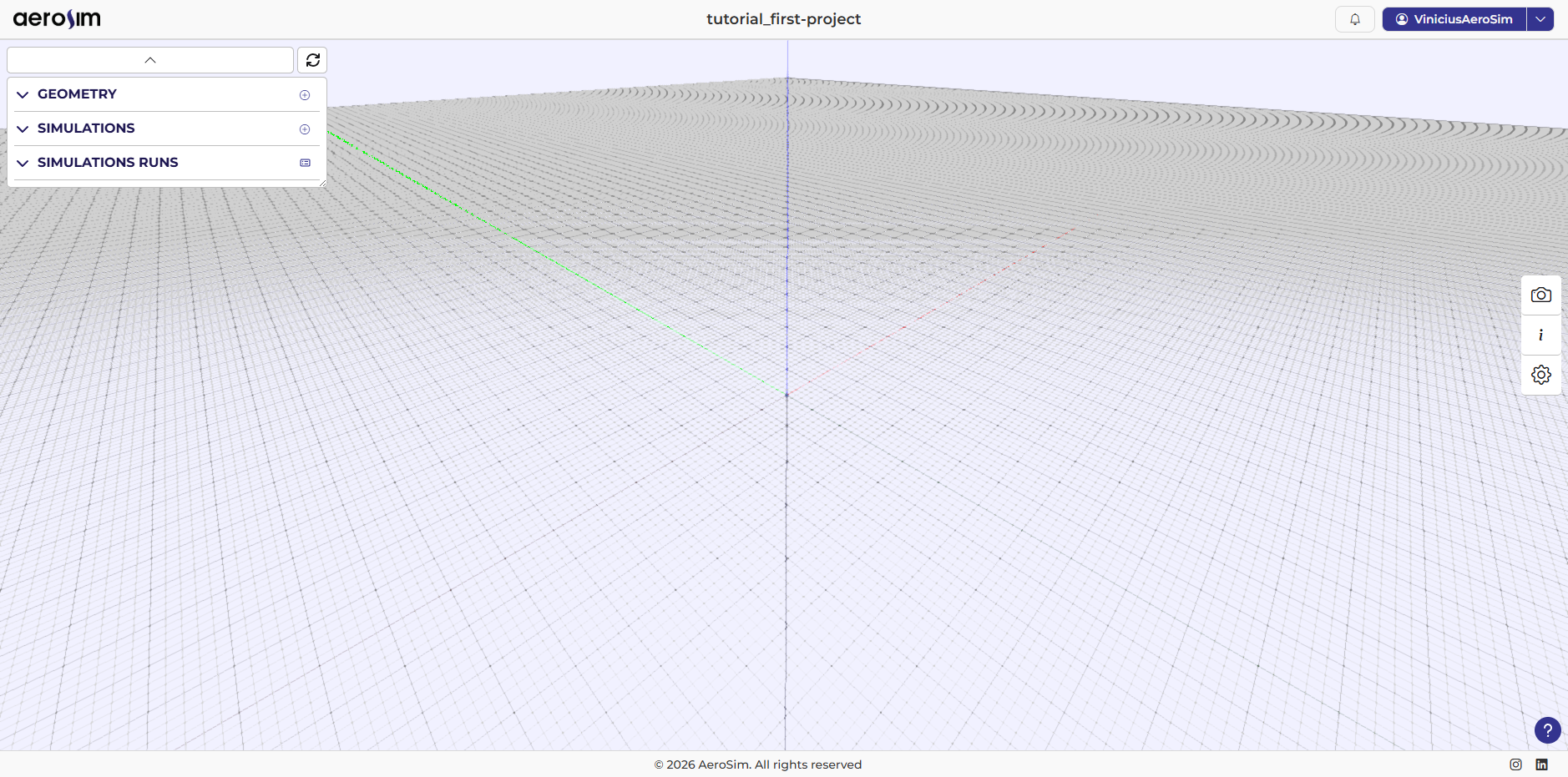
An empty project.
Geometry
You can generate a geometry or upload one. Once added, the geometries are available for any simulation in the project.
Importing
Download the tutorial geometry file:
Ground - a plane representing the ground
Click on Import Geometry and load the Terrain file provided. After importing, the geometries are validated (format, integrity, and compatibility with the solver) and added to the project if they are correct.
Generating
Click Generate Geometry and select option Cube in the dropdown and set the following parameters:
Length: 1 m
Width: 1 m
Height: 1 m
Target Edge Size: 0.04 m
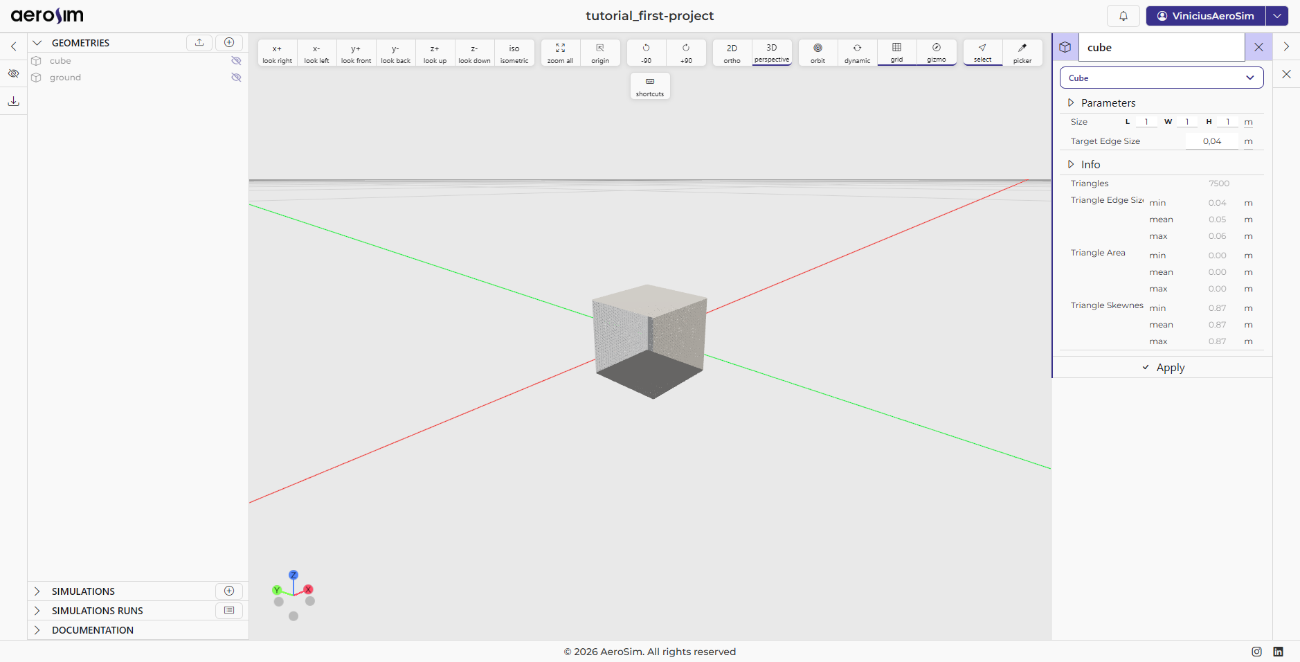
Creating a geometry.
Note
The mesh will be divided in a way that makes the triangles more equilateral. Therefore, we define a target value for the length of the triangle’s edge, and not the final length itself.
Simulation
After importing the geometries, create a new simulation and start configuring it.
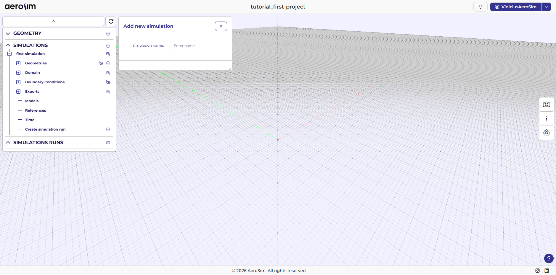
Creating the simulation.
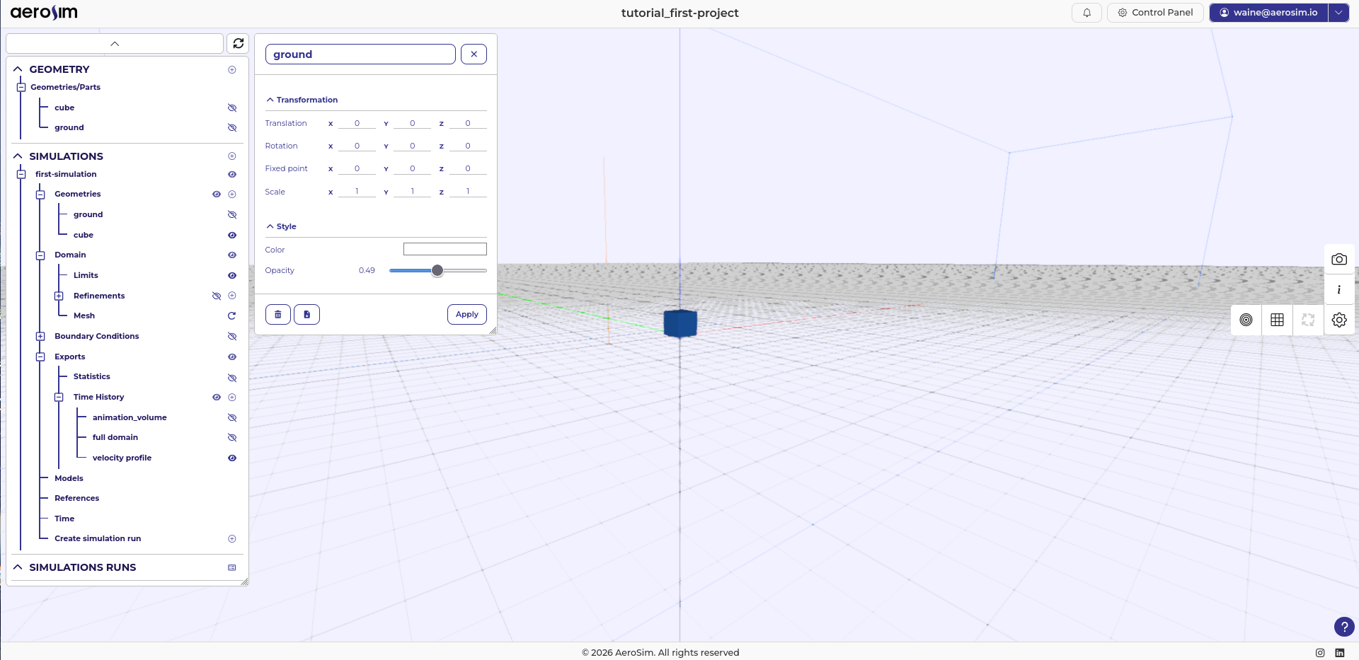
Geometries
Add the ground geometry first, then the cube. In the cube object set all three Scale components to 30 so the cube measures 30 m along each edge. Also set the translation in z to 15 m, so the bottom face sits at \(z = 0\).
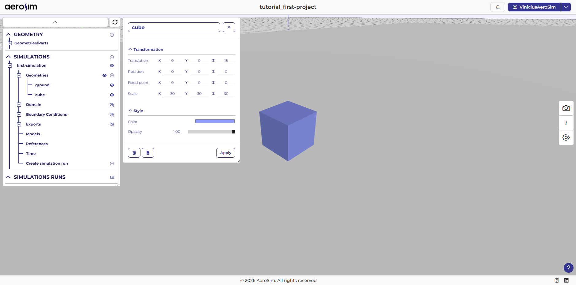
Adding geometries to the simulation.
Tip
You can change geometry colors and global illumination to improve visualization.
Domain
The domain is the computational region where the governing equations are solved. Make it large enough that the boundaries do not interfere with the area of interest.
Set the domain dimensions:
Length: 2500 m - long enough to place boundaries far from the model
Width: 600 m
Height: 600 m
X (origin offset): -500 m
Y: 0 m
Z: -51 m - placing the domain floor 51 m below ground level to keep the bottom boundary away from the ground plane
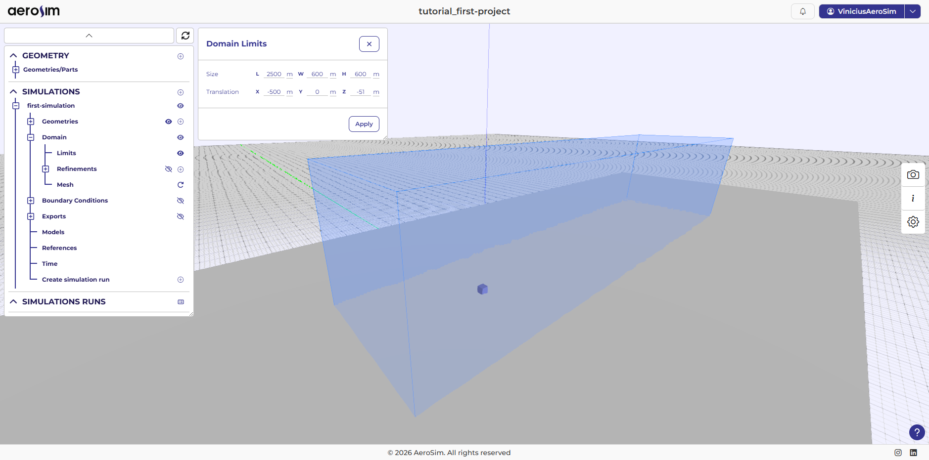
Domain configuration.
Refinements
Refinements locally increase mesh resolution to better capture flow gradients and features. Target Refinement is the desired local cell size (smaller -> finer). Max Cell Size caps how large cells can grow inside the refinement region.
Create two refinements:
cube refinement (Body refinement)
Target Refinement: 0.6 m
Max Cell Size: 1.0 m
Target body: cube
Thickness (inner): -2 m - negative value means the refinement zone extends slightly inside the body surface, which ensures full coverage of the IBM diffusive layer
Thickness (outer): 6 m - outer layer that transitions to the coarser mesh
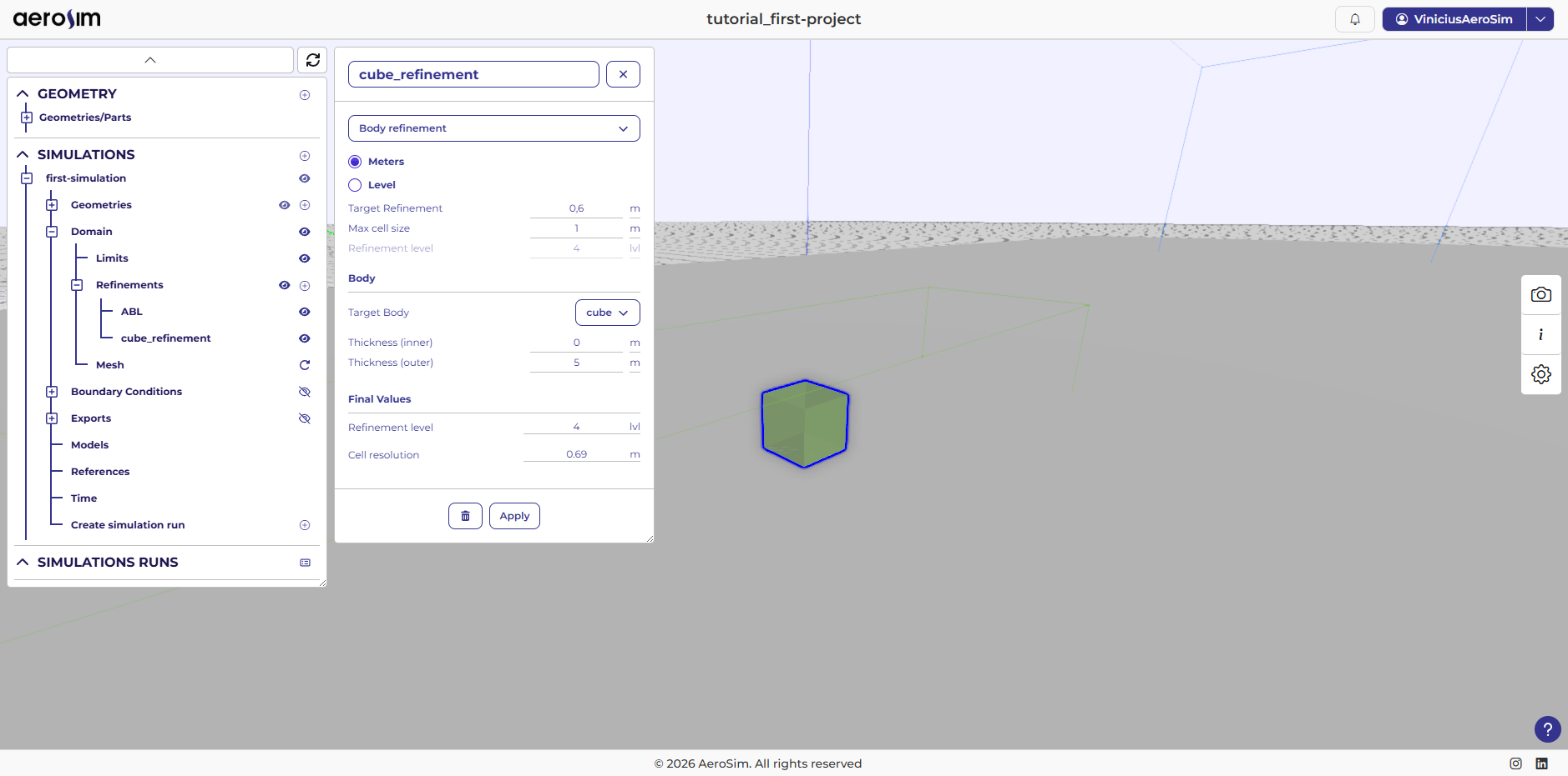
Cube refinement configuration.
ABL (Box refinement) - improves resolution of the atmospheric boundary layer near the cube
Target Refinement: 1.5 m
Max Cell Size: 2.5 m
Volume coordinates (Min): (-500, -60, -10) m
Volume coordinates (Max): (200, 60, 60) m
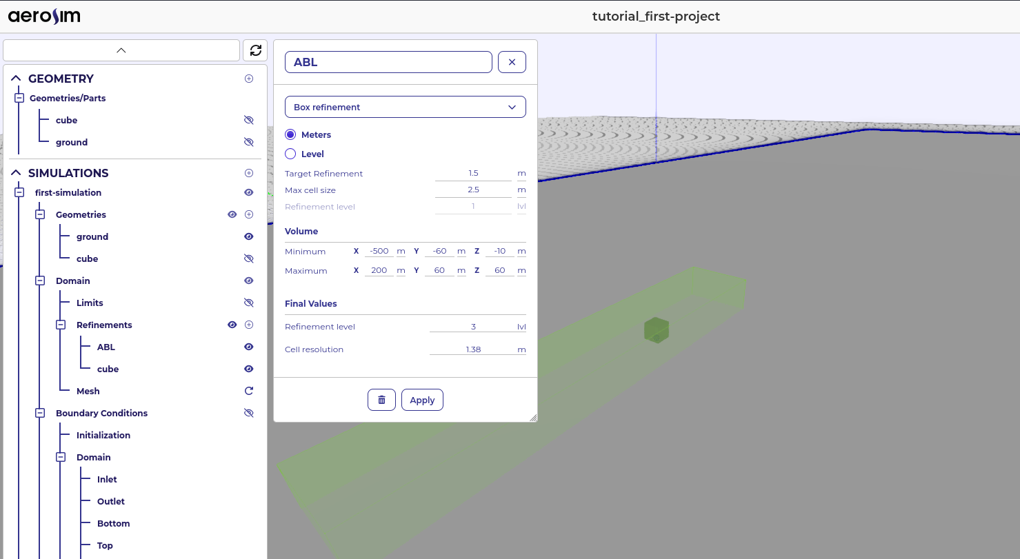
Atmospheric Boundary Layer (ABL) refinement.
Mesh
Set Baseline Resolution = 11. This is a global control for overall mesh density - a higher value produces a finer mesh but increases computation time.
After clicking Apply, a mesh preview will appear. If it does not update automatically, refresh the scene tree.
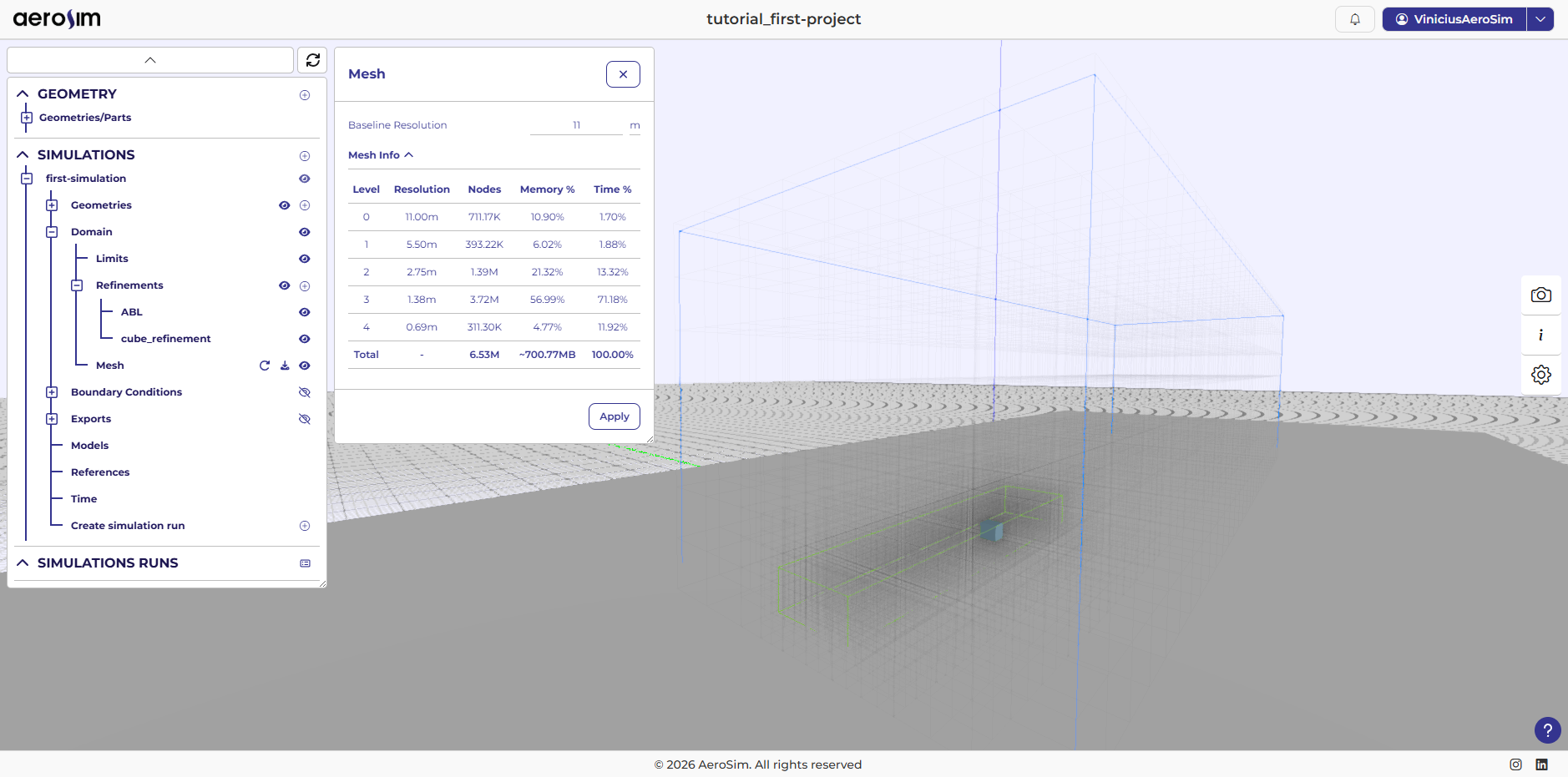
Generated mesh.
Note
For this tutorial the mesh update is fast; larger cases may take longer. To avoid UI slowdowns, update the visualization manually after changes.
Boundary conditions
Boundary conditions (BCs) define the flow behavior at domain boundaries and on bodies.
Initialization
Initial Velocity: 10 m/s - starting velocity for the entire domain
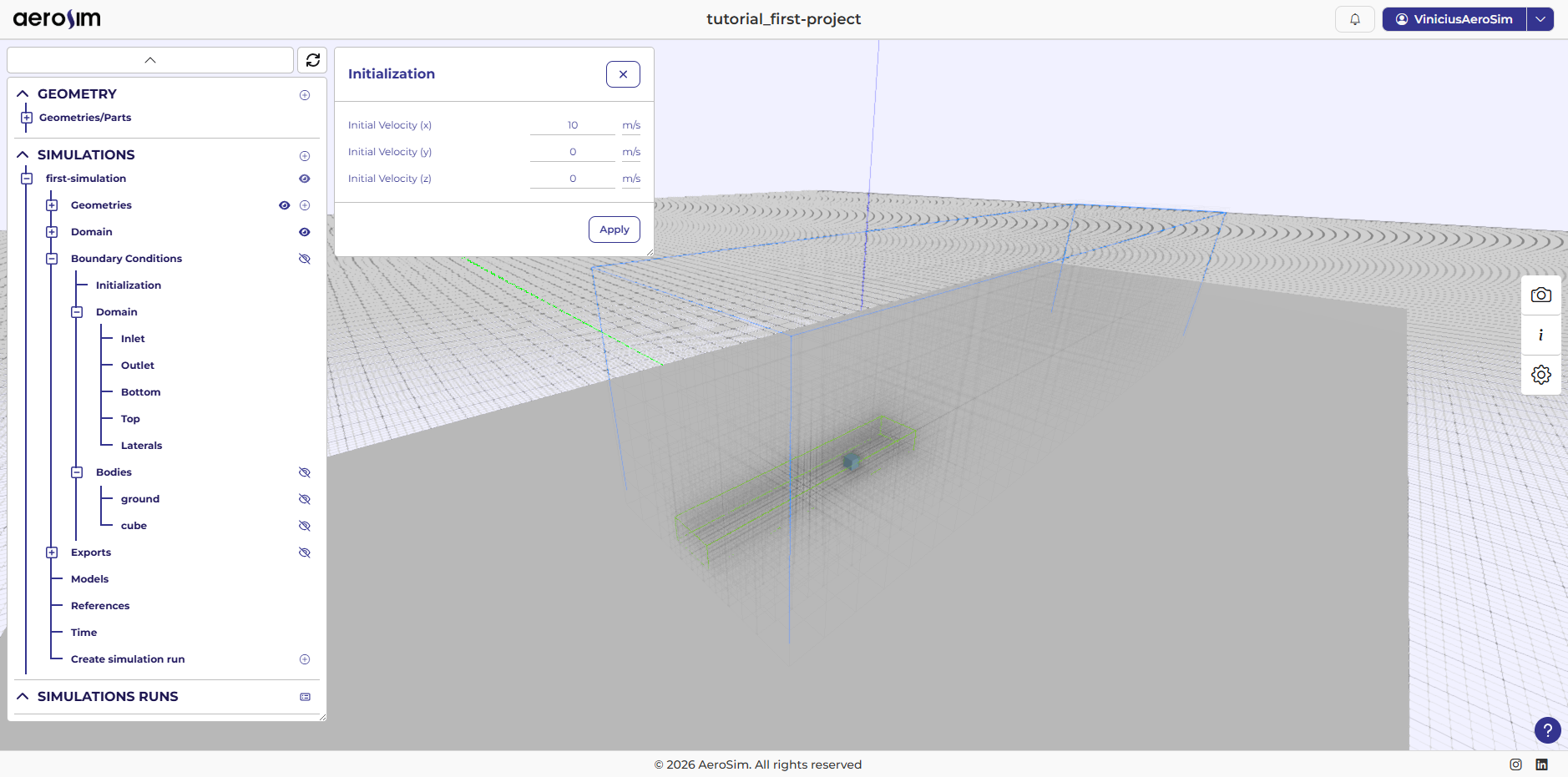
Initialization settings.
Inlet
In the Inlet section, select SEM as the inlet type and enable From Generator. Set the following parameters:
Roughness length: 0.05 m - ground roughness used by the ABL generator
Target Velocity: 10 m/s - desired inflow speed
Reference height: 30 m - height at which the target velocity is specified
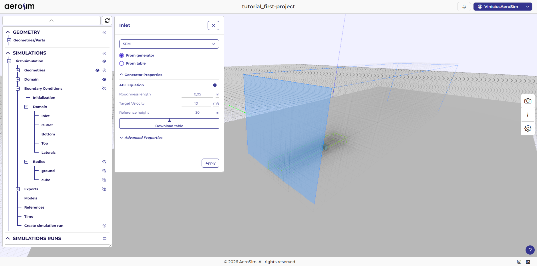
Inlet configuration.
Outlet
Outlet boundary condition: Fixed Pressure - set to 0 Pa
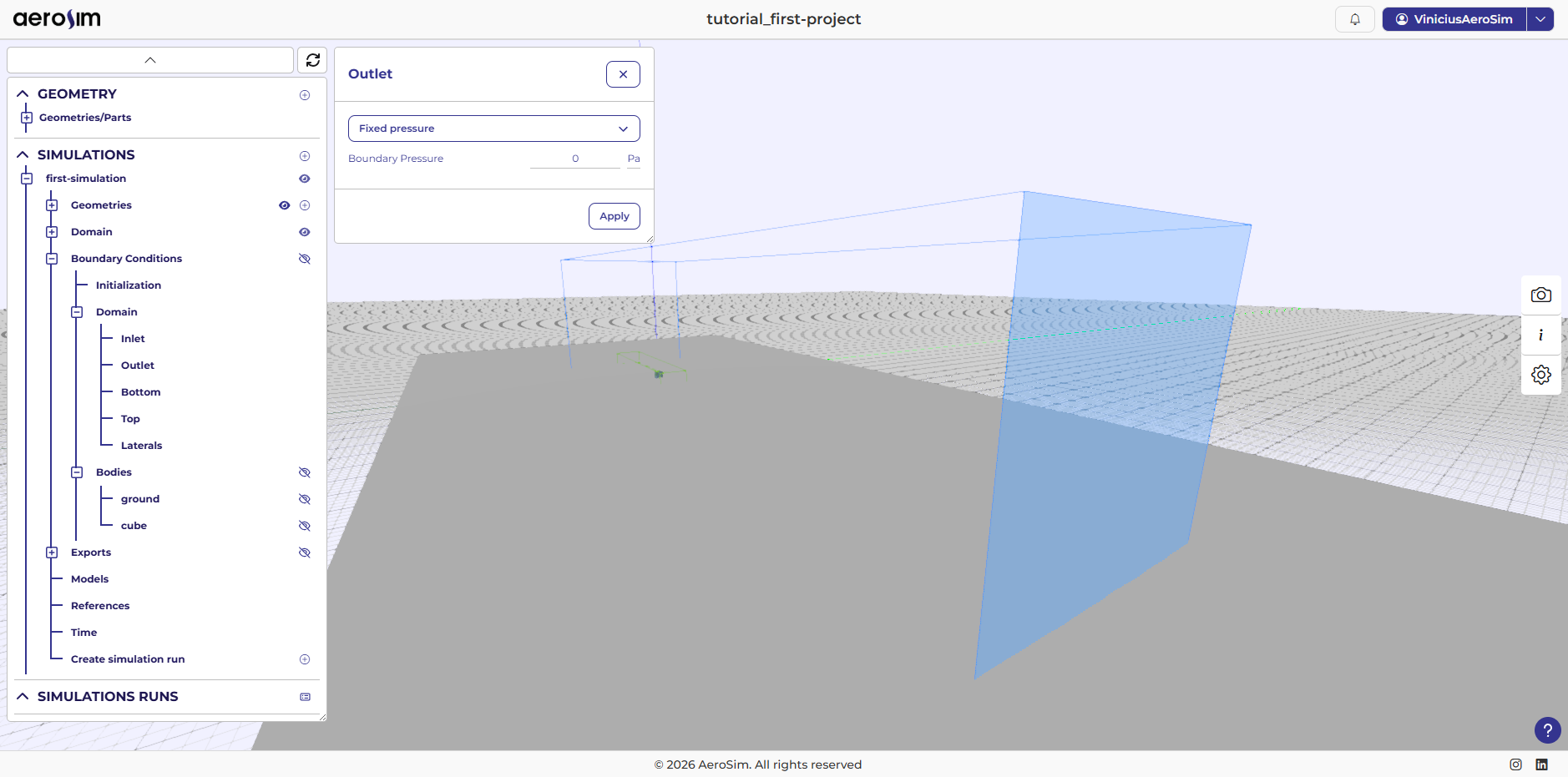
Outlet configuration.
Laterals, Top and Bottom
For the laterals, top and bottom, leave the default values. Lateral and top use Neumann and Bottom uses no-Slip.
Bodies
Configure each geometry with appropriate body settings:
Ground: Wall + ABL Wall Model
Roughness Length: 0.05 m
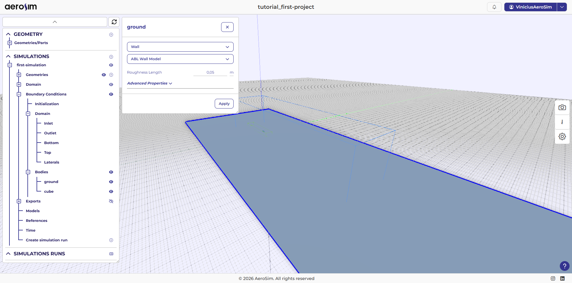
Ground body configuration.
Cube: Wall + No‑Slip
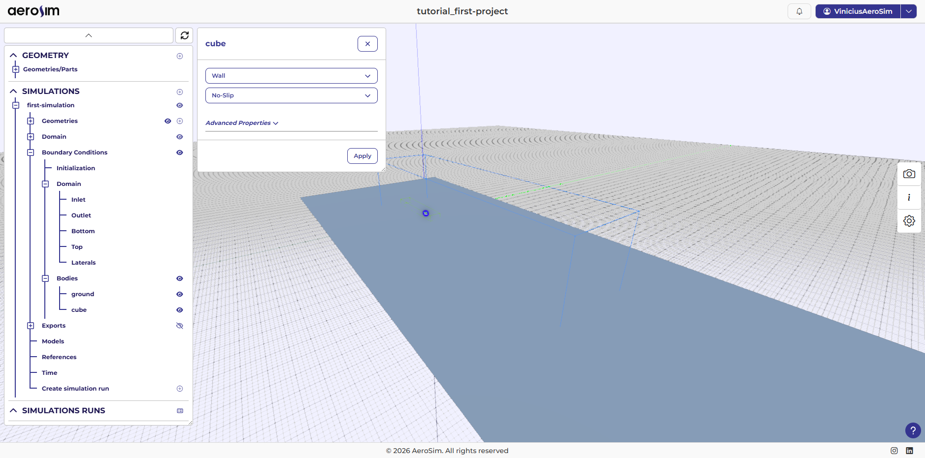
Cube body configuration.
Exports
Exports control what data is written to disk for post‑processing.
Domain statistics
Enable domain statistics.
Sampling volume: (-500, -100, 0) to (200, 100, 100) m
Sampling Period: 1 s - sample every second of simulated time
Initial Time: t = 120 s - start sampling after the flow has developed
Export fields: Pressure, Velocity Ux, Velocity Uy, Velocity Uz
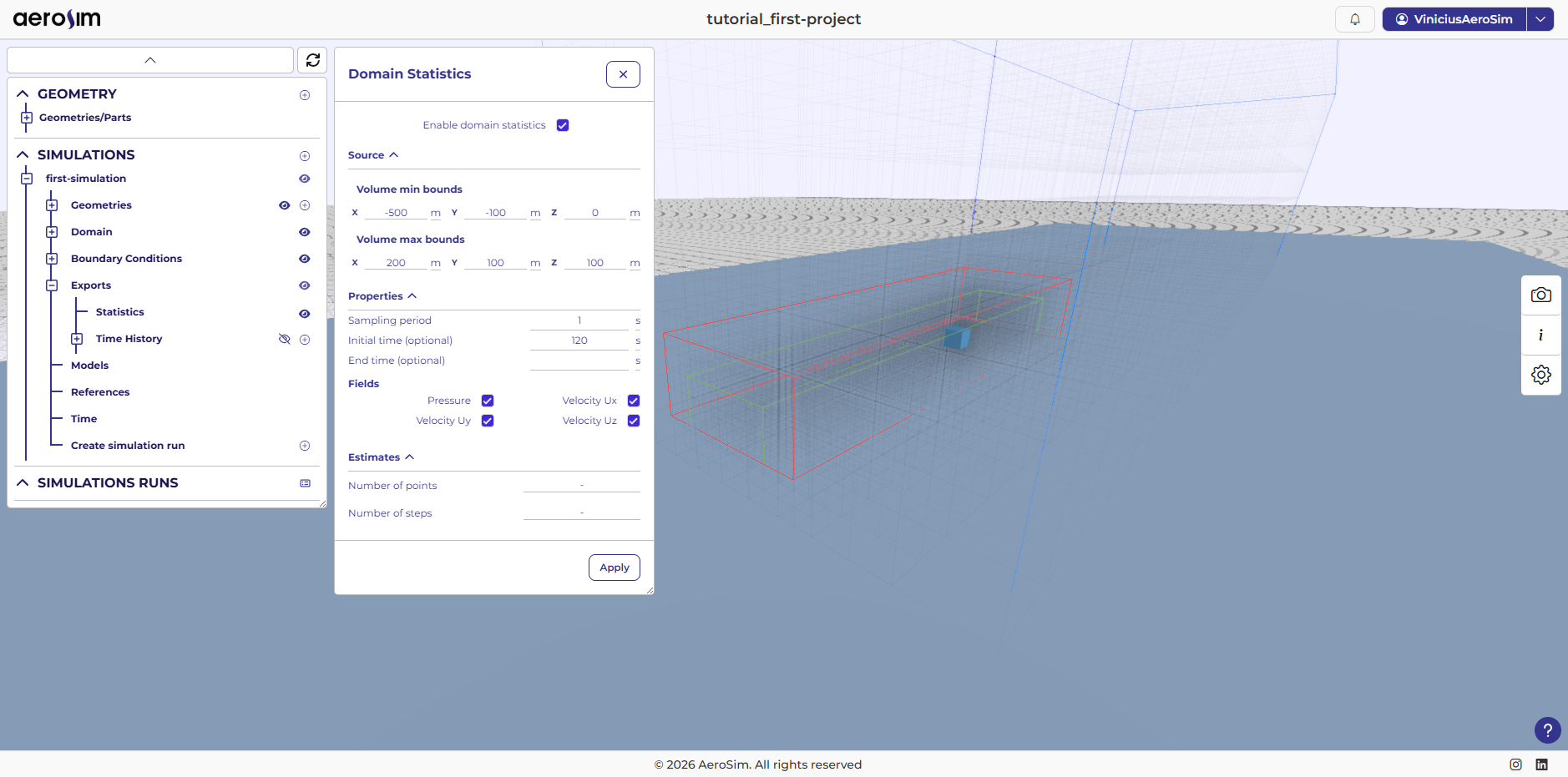
Statistics configuration.
At the end of the simulation, time-averaged statistics over the sampling volume are exported.
Animation Volume
A volume export captures the full 3D flow field at each saved time step, producing files you can animate in ParaView to see how the flow develops around the cube.
Use a tighter bounding box focused around the cube, and limit the time window to keep the output size manageable:
Volume: (-100, -100, 0) to (300, 100, 100) m
Sampling Period: 0.3 s
Initial Time: t = 120 s
Final Time: t = 180 s - a 60 s window gives roughly 200 snapshots, enough for a smooth animation
Export fields: Pressure, Velocity Ux, Velocity Uy, Velocity Uz
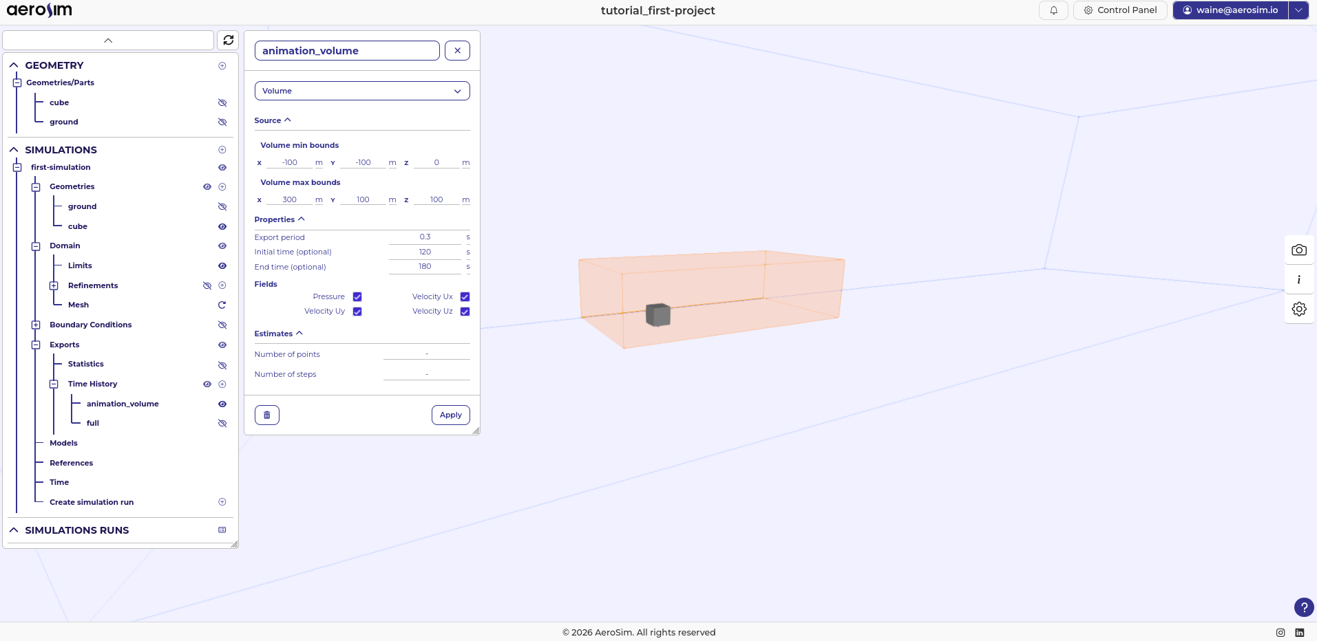
Animation volume export configuration, showing the bounding box around the cube.
Full Domain Export
A full-domain snapshot is useful for a quick sanity check of the overall flow field. Because it covers the entire domain at low frequency, it adds little storage overhead.
Volume: (-500, -300, -50) to (2500, 300, 550) m - extends beyond the domain boundaries without issue
Sampling Period: 100 s - produces about 7 snapshots over the full 720 s run
Leave Initial Time and Final Time empty to cover the entire simulation
Export fields: Pressure, Velocity Ux, Velocity Uy, Velocity Uz
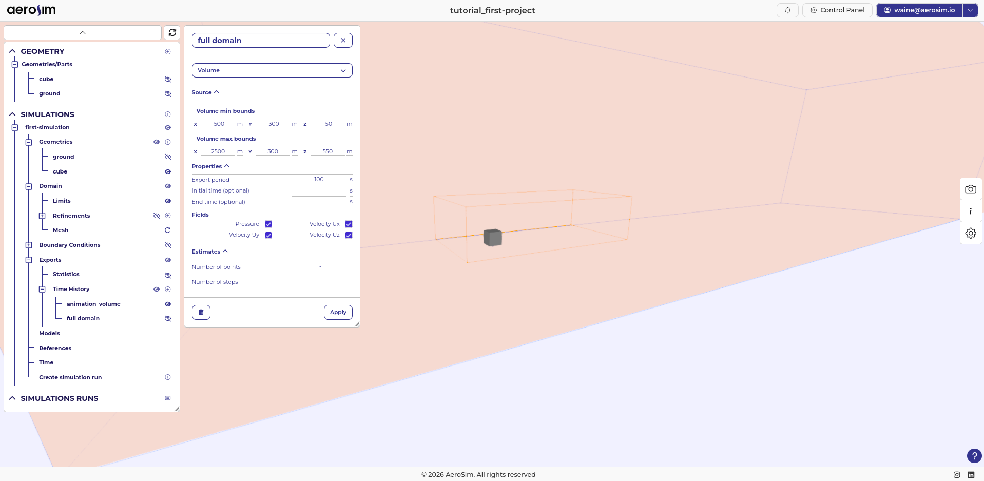
Full domain export configuration, covering the entire computational domain.
Pressure on Cube
A body export captures pressure on the cube surface, letting you calculate statistics and visualize pressure distributions.
Set up a body export for the cube as:
Body:
cubeNormal offset: 1.5 m
Sampling Period: 0.3 s
Initial Time: t = 120 s
Export fields: Pressure
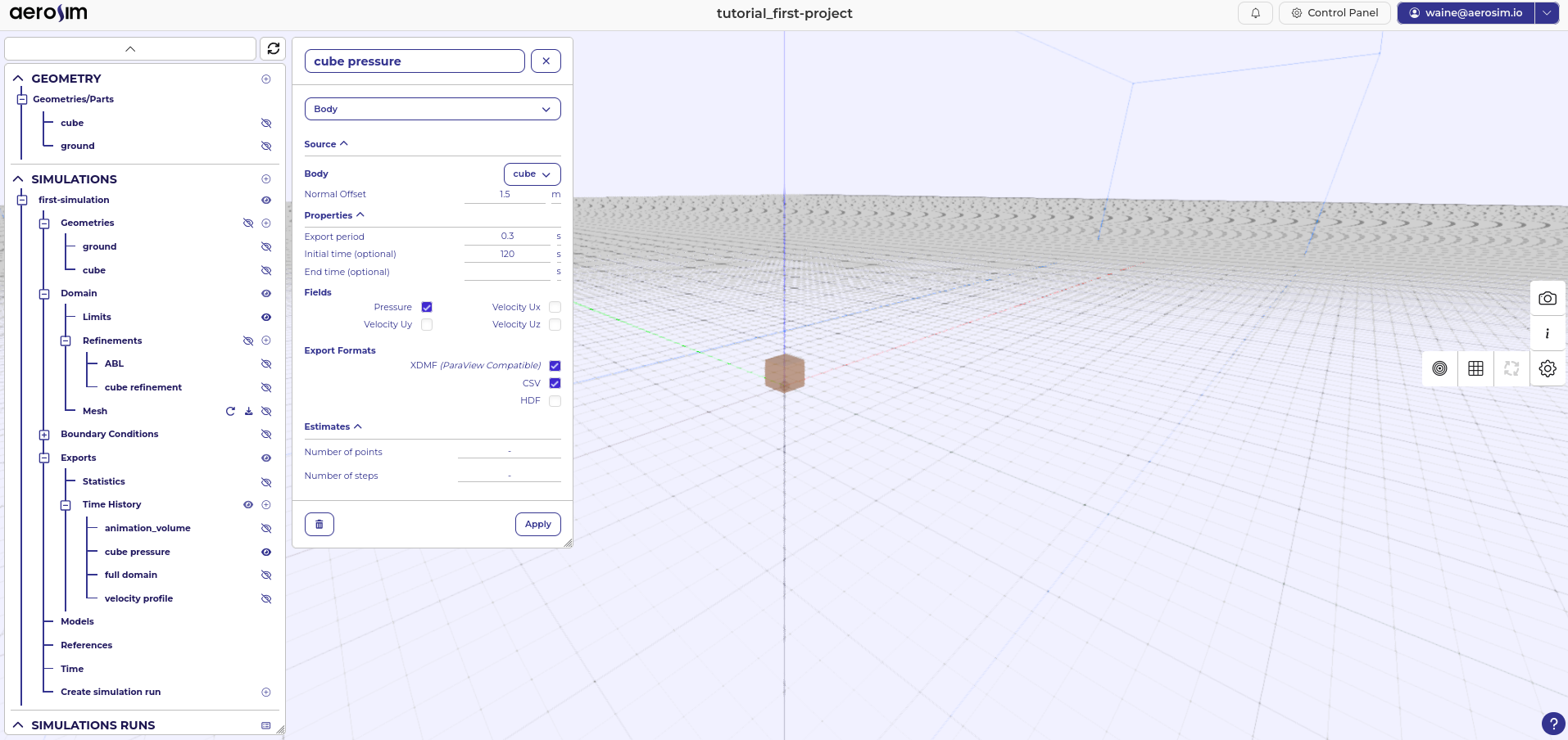
Cube pressure export configuration.
Important
For pressure on bodies, it’s important to export with a normal offset of at least 2 times the body resolution, to avoid numerical disturbances caused by the IBM boundary conditions at the cube. In this case the cube meshed cell size is approximately 0.7 m (slightly above the 0.6 m target), so the normal offset should be higher than 1.4 m.
Velocity line
A profile line samples the velocity at a sequence of points along a vertical line, letting you check the incoming flow profile after the simulation.
Set up a vertical line upstream of the cube:
Start point: (-100, 0, 0) m - upstream of the cube, sampling the incoming flow profile
End point: (-100, 0, 200) m
Number of points: 201
Sampling Period: 0.3 s
Initial Time: t = 120 s
Export fields: Velocity Ux, Velocity Uy, Velocity Uz
Velocity line export configuration, sampling the incoming flow profile upstream of the cube.
Only \(U_x\) is used for the incoming flow profile check.
Reference properties
Set the reference physical properties:
Fluid Viscosity: 0.03675 Pa·s
Fluid Density: \(\rho\) = 1.225 kg/m^3
Reference pressure: 0 Pa
Note
The viscosity value is not the physical value for air. In AeroSim, it is chosen to set a target Reynolds number for the simulation. For this tutorial case (\(U = 10\,\text{m/s}\), \(L = 30\,\text{m}\), \(Re = 10^4\)):
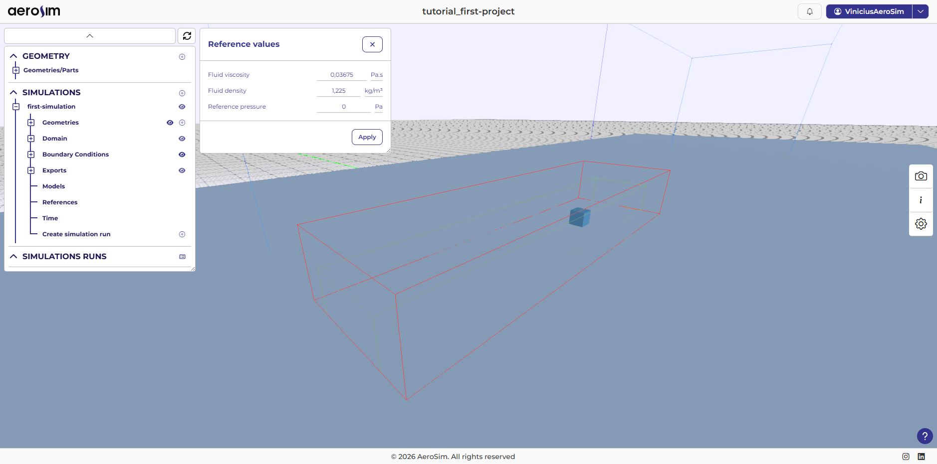
Reference properties.
Time
Set the simulation time controls:
Total time: 720 s
CFL max: 0.1 - maximum CFL number used by the time integrator
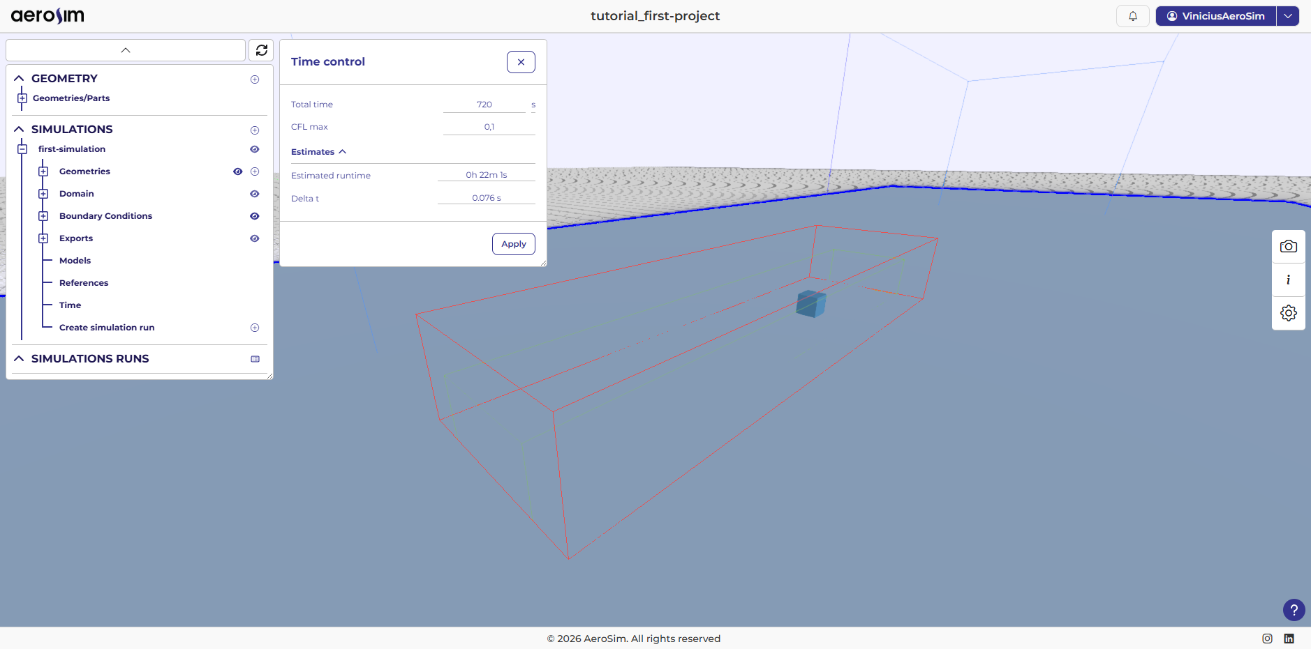
Time configuration.
Next steps
The simulation is now configured. Proceed to Running the simulation.