Surface Line Probe

A common post-processing task is to extract field values along a line that follows a body surface. For example, measuring the pressure coefficient \(c_p\) around the perimeter of a building at a given height. Unlike a straight probe through empty space, this line traces the geometry itself - walking over each face the surface has in a given direction.

The technique works by intersecting the surface mesh with a cutting plane. The plane is oriented so that its intersection with the body produces a polyline in the desired direction. Field values are then sampled along that polyline.

---

Concept

Given a starting point on the surface and a walking direction (e.g. \(\hat{x} = (1, 0, 0)\)), the goal is to obtain a line that travels along the surface in that direction until it reaches the edge of the body.

This is achieved by defining a cutting plane that:

1. Passes through the starting point.

2. Contains the walking direction vector.

3. Is oriented so that the plane-surface intersection produces the desired path.

The plane normal is perpendicular to the walking direction. For a horizontal traverse in the \(x\)-direction, the cutting plane is vertical with normal \(\hat{n} = (0, 1, 0)\), positioned at the \(y\)-coordinate of the starting point. The intersection of this plane with the surface mesh yields a polyline that follows every face of the body at that \(y\)-position.

Walking direction	Plane normal	What it traces
\(x\)-direction \((1,0,0)\)	\((0,1,0)\) at the desired \(y\)	Longitudinal cut along the body
\(y\)-direction \((0,1,0)\)	\((1,0,0)\) at the desired \(x\)	Lateral cut along the body
Horizontal at height \(z\)	\((0,0,1)\) at the desired \(z\)	Perimeter of the body at a fixed height

Note

A horizontal cutting plane (normal \((0,0,1)\)) at a fixed height is the most common choice for buildings. It traces the full perimeter of the cross-section at that elevation, which is exactly the path used to plot \(c_p\) distributions around a structure.

---

ParaView Workflow

Step 1: Load the Surface Data

Open the body surface file in ParaView (e.g. bodies.body_Cp body.xdmf). If you have already computed \(c_p\) using the Pressure Coefficient Measurement workflow, the Cp field will be available alongside pressure.

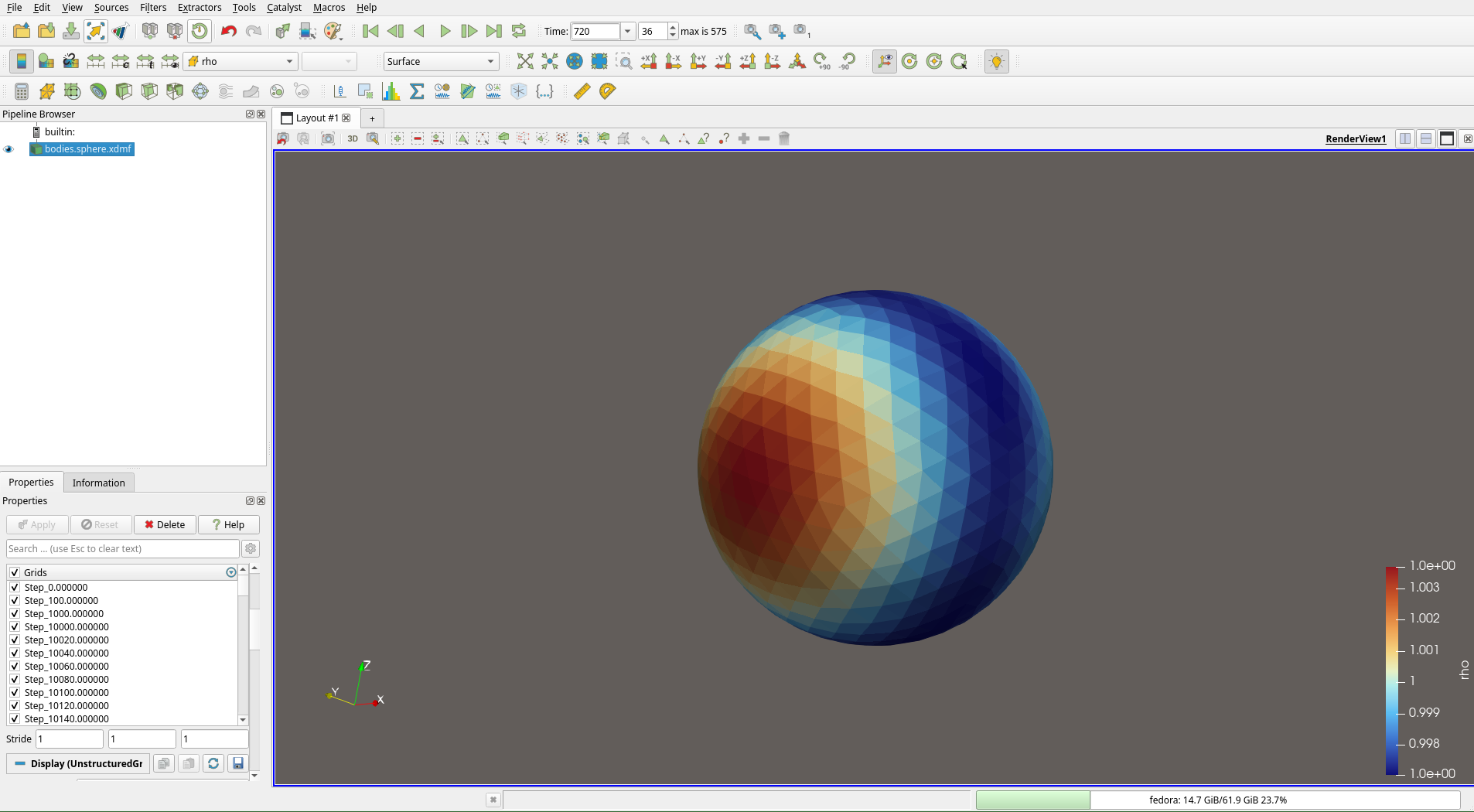
Body surface loaded in ParaView, coloured by pressure (cell data).

Step 2: Convert Cell Data to Point Data

AeroSim body exports store field values per triangle (cell data). The intersection filter produces point data along the curve, so the cell fields must be converted first.

1. Select the surface dataset in the Pipeline Browser.

2. Apply Filters -> Cell Data To Point Data (or press Ctrl+Shift+D and search for “Cell Data To Point Data”).

3. Click Apply.

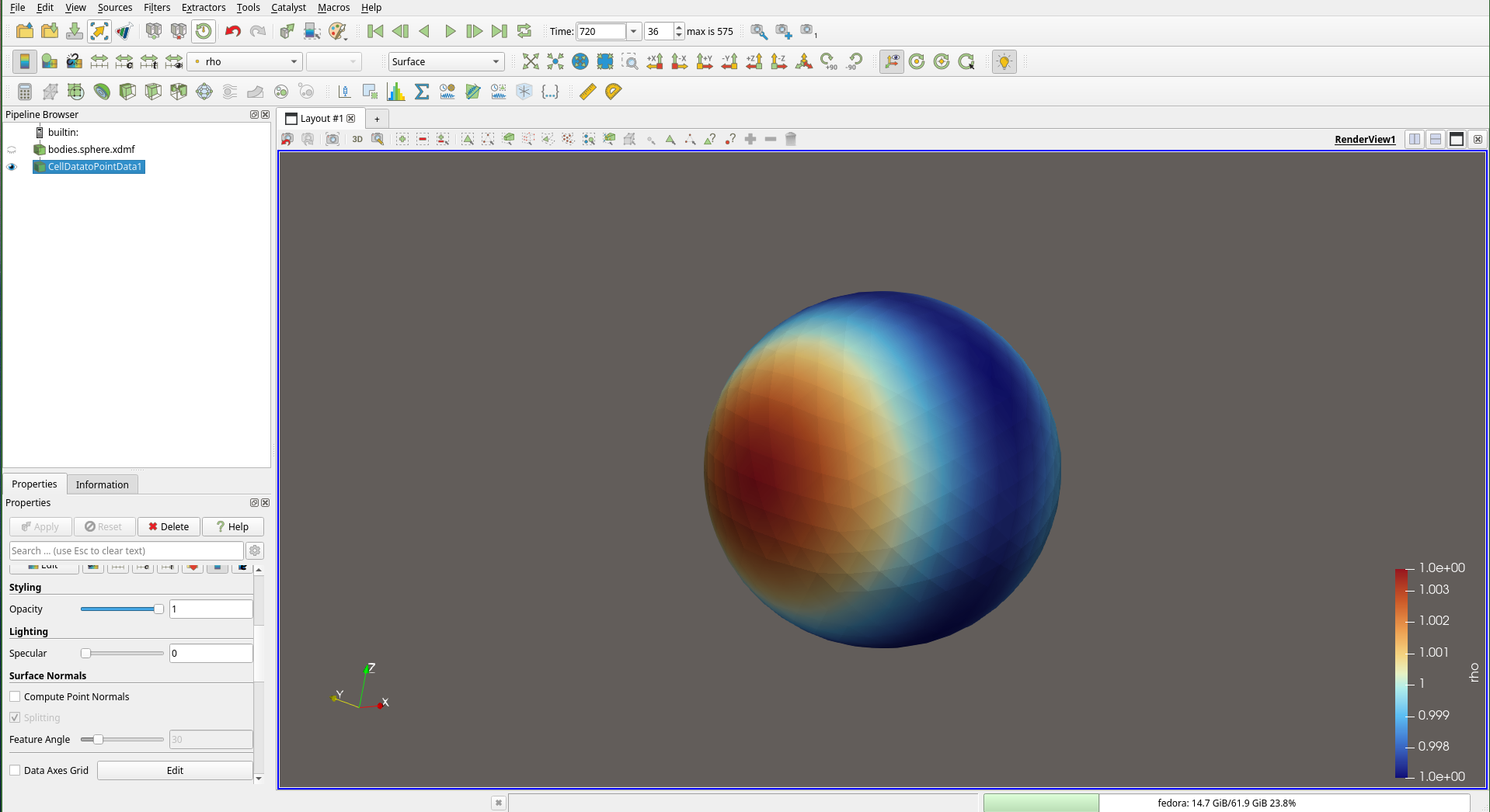
Surface after applying Cell Data To Point Data. The field is now stored at mesh vertices and can be interpolated along the intersection curve.

Step 3: Apply Plot On Intersection Curves

The Plot On Intersection Curves filter combines the surface extraction, plane intersection, and arc-length computation into a single step.

1. Select the Cell Data To Point Data output in the Pipeline Browser.

2. Go to Filters -> Data Analysis -> Plot On Intersection Curves (or press Ctrl+Shift+D and search for “Plot On Intersection Curves”).

3. In the Properties panel, set the Slice Type to Plane.

4. Set the Origin to a point where you want the cut to pass. For a horizontal cut at mid-height of a building of height \(H\), set the origin \(z\)-coordinate to \(H/2\).

5. Set the Normal to define the cutting plane orientation. For a horizontal cut, use \((0, 0, 1)\).

6. Click Apply.

ParaView will display a line chart of the selected field versus arc length along the intersection curve. The 3-D view shows the intersection polyline on the surface, so you can visually confirm the cut location.

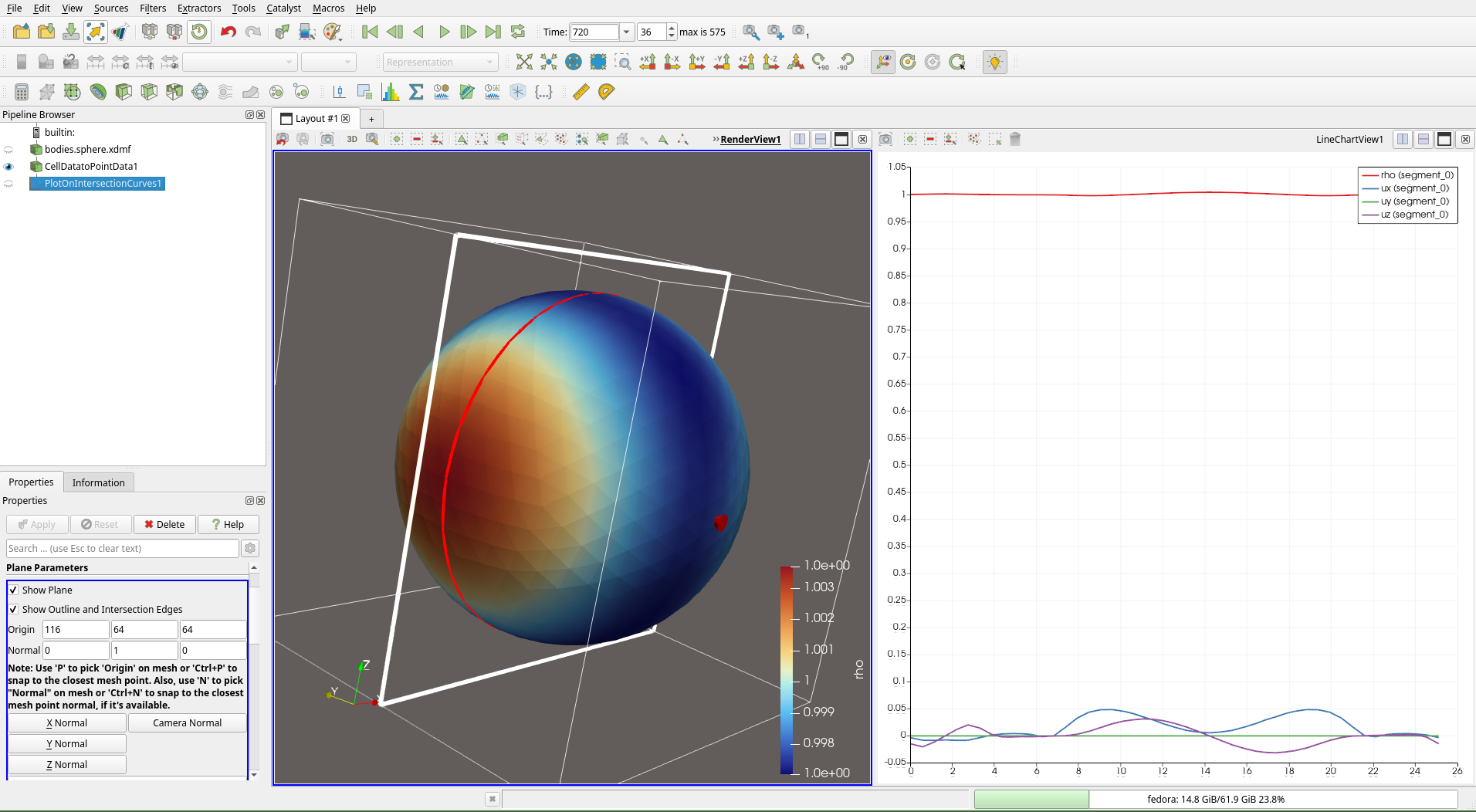
Plot On Intersection Curves applied to the surface. The 3-D view shows the cutting plane and the intersection polyline (red), while the line chart on the right displays all available fields.

In the Series Parameters section of the Properties panel, toggle individual fields on or off to isolate the variable of interest.

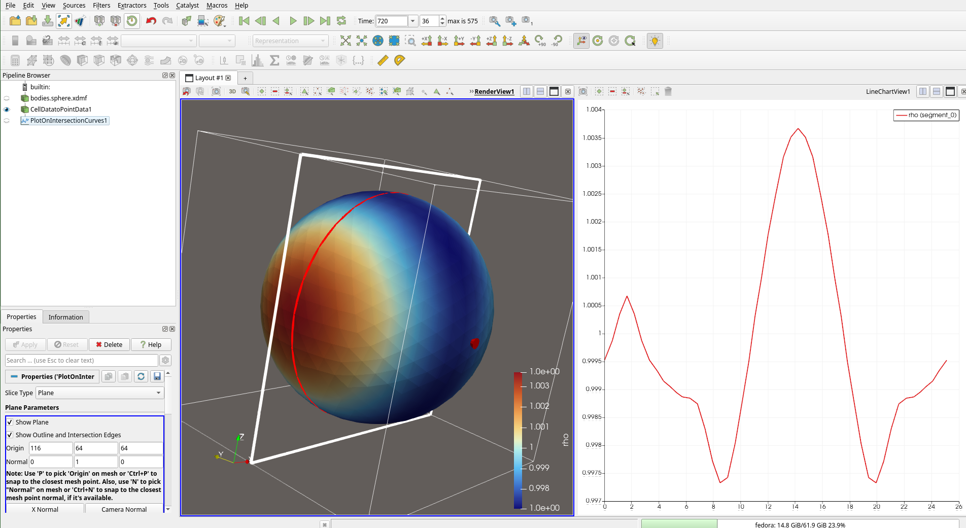
The same intersection with only the pressure field selected, giving a clean arc-length profile.

Step 4: Export the Data

1. Select the Plot On Intersection Curves output in the Pipeline Browser.

2. Go to File -> Save Data… and choose CSV format.

3. The exported CSV will contain arc_length, the coordinates of each point on the polyline, and all field values at those locations.

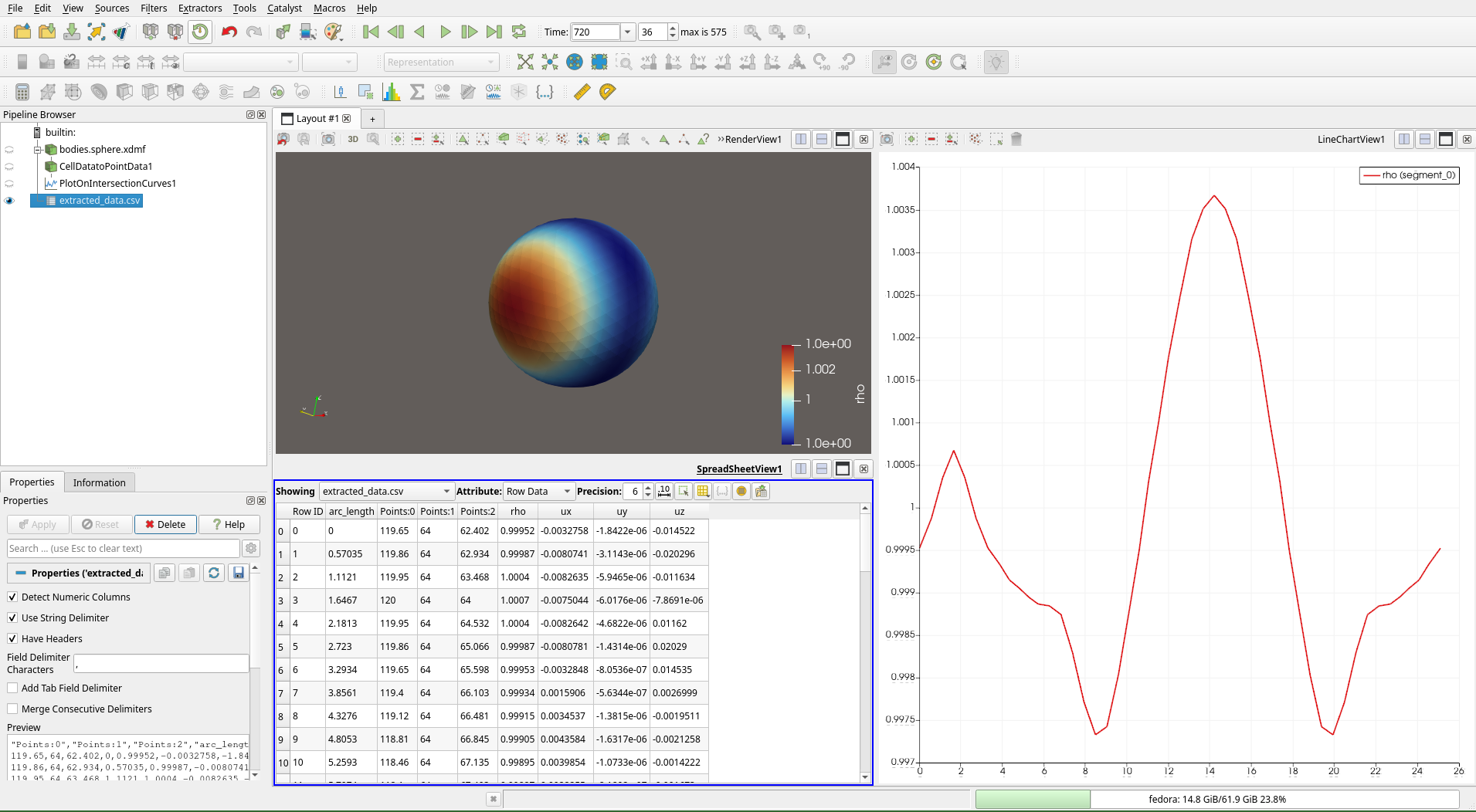
Spreadsheet view showing the exported point data with coordinates, arc length, and field values.

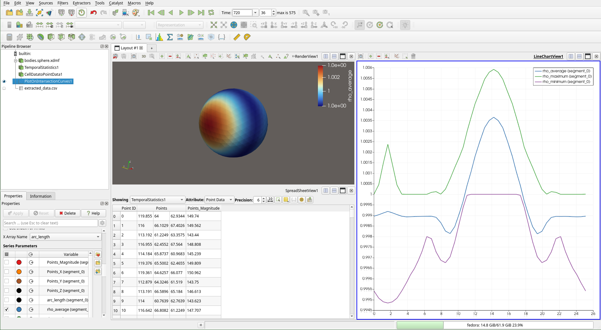
Final line chart with multiple fields plotted against arc length along the intersection curve.

---

Practical Example: \(c_p\) Around a Cube

A standard validation exercise is to measure \(c_p\) at mid-height around a surface-mounted cube and compare it with wind tunnel data.

Setup:

• Cube of side \(H\) centred at the origin.

• Horizontal cutting plane at \(z = H/2\) with normal \((0, 0, 1)\).

• Field: Cp (computed beforehand using the Pressure Coefficient Measurement workflow).

The slice produces a closed rectangular polyline that traces the four faces of the cube at mid-height. The exported \(c_p\) values show the windward stagnation, side-face suction, and leeward wake region in sequence.

Tip

When comparing with experimental data, normalise the arc length by the characteristic length (e.g. the cube side \(H\)) so that both datasets share the same horizontal axis.