Pressure Coefficient Measurement¶

The pressure coefficient \(c_p\) is a dimensionless quantity that characterises the local pressure distribution on a body’s surface relative to the undisturbed flow. Because it removes the dependence on wind speed and fluid density, \(c_p\) results from different simulations or wind tunnel experiments can be compared directly, and they form the input to structural load calculations.

This guide covers how to configure the pressure exports in AeroSim and how to compute \(c_p\) as a time series from the simulation output.

Definition¶

The pressure coefficient is computed at each instant in time:

\[ c_p(t) = \frac{p(t) - p_\infty(t)}{q} \]

where:

Symbol	Quantity	Notes
\(p(t)\)	Local pressure on the body surface	Exported as a time series from the body surface monitor
\(p_\infty(t)\)	Reference (free-stream) static pressure	Exported from a probe point above and away from the structure
\(q\)	Dynamic pressure \(\tfrac{1}{2}\rho\,U_H^2\)	Uses the mean velocity \(U_H\) at the height of interest

Important

Both \(p(t)\) and \(p_\infty(t)\) are time series. Using only the time-mean of the reference pressure would corrupt the instantaneous \(c_p\) signal and distort peak statistics. The subtraction must be done point-by-point in time.

The impact of using a constant \(p_\infty\) versus a time-varying \(p_\infty(t)\) is visible in the RMS of \(c_p\). The figure below compares both approaches on the same case, showing how treating the reference as constant artificially inflates the RMS on the surface.

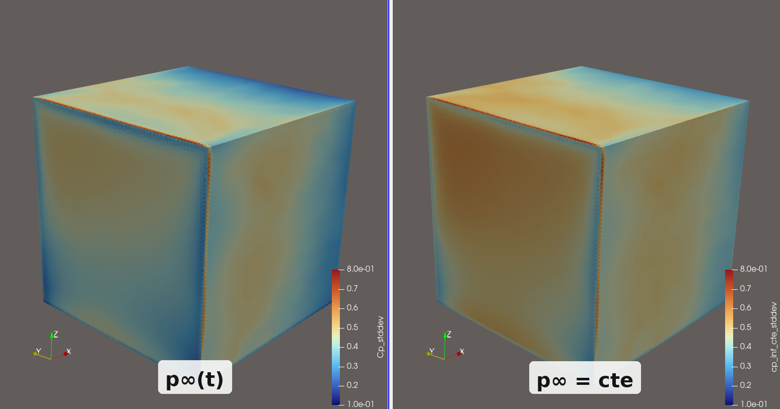
../../_images/04-cp-inf-comparison.png — RMS of \(c_p\) computed with a time-varying \(p_\infty(t)\) (left) versus a constant \(p_\infty\) (right). Using a constant reference inflates the RMS across the surface.¶

Setting Up the Exports¶

Two exports must be configured before running the simulation: a body surface export that records pressure on the structure, and a reference point export that records the free-stream static pressure.

Body Surface Export¶

In AeroSim, add a body export and set the Pressure field. The critical parameter is normal_offset.

Set normal_offset = 2 * body_ref to displace the sampling plane two lattice cells outward along the surface normals, placing all probes in the fully resolved fluid region.

Note

body_ref is the mesh resolution assigned to the body geometry (in metres). If the body is refined to \(\Delta x\) = 0.5 m, then normal_offset = 1.0 m.

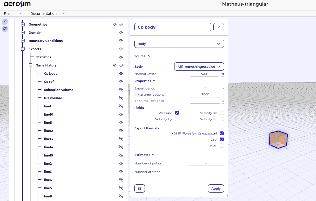
../../_images/01-body-export-setup.png — Body export configuration in AeroSim, showing the Pressure field selected and `normal_offset` set to `2 * body_ref`.¶

Note

Why the offset is needed:

AeroSim represents solid surfaces using the Immersed Boundary Method (IBM). Inside the IBM near-wall zone (~1.5 lattice cell from the geometry surface), pressure values are affected by the interpolation/spreading rather than resolved by the LBM stencil. Sampling at the geometry surface itself would therefore yield values that are partially numerical artefact rather than physical surface pressure. The offset moves the probes past this zone while remaining close enough to be representative of the surface pressure.

Reference Point Export¶

Add a point export and place the probe at a location that is:

Height: at least \(\max(2H,\,400\,\text{m})\) above the roof, where \(H\) is the building height. This ensures the point is above the pressure disturbance induced by the roof.
Horizontal position: directly above the building centroid, or sufficiently far upstream/lateral that the building blockage does not affect the local mean pressure.

The probe captures the instantaneous atmospheric static pressure \(p_\infty(t)\), which fluctuates in time with the turbulent flow but carries no building-induced component.

Warning

If the reference point is placed too close to the structure, the building’s pressure field will contaminate \(p_\infty(t)\) and bias all \(c_p\) values. The \(\max(2H,\,400\,\text{m})\) height guideline is a minimum; increase it if the flow is affected by terrain or buildings at that height.

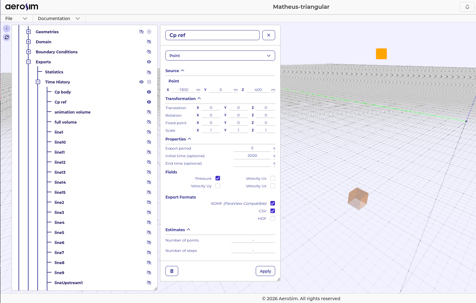
../../_images/02-reference-point-setup.png — Reference point positioned at \(z \geq \max(2H,\,400\,\text{m})\) above the building, well outside its pressure influence zone.¶

Important

Both exports must share the same time range and sampling interval. A mismatch in timesteps will make the per-instant subtraction \(p(t) - p_\infty(t)\) impossible.

Computing \(c_p\)¶

After the simulation completes, download the body and reference point files:

bodies.body_Cp body.h5 / bodies.body_Cp body.xdmf
points.point_Cp ref.h5

The script below reads both files, computes \(c_p(t)\) for every surface triangle at every timestep, writes the result back into the body HDF5 file as a new dataset group cp/, and patches the XDMF descriptor so that the Cp field is immediately available when the file is opened in ParaView. The values of rho, U_H, and \(q\) are stored as attributes on the cp/ group so that downstream scripts (e.g. the Structural Load workflow) can read them automatically.

Note

The script requires h5py and NumPy. Install them with pip install h5py numpy if not already available.

Download compute_cp.py

import h5py
import numpy as np
import xml.etree.ElementTree as ET
from pathlib import Path

# ---------------------------------------------------------------
# Parameters - edit these to match your simulation
# ---------------------------------------------------------------
rho = 1.225   # kg/m^3 - fluid density
U_H = 1.6   # m/s    - mean velocity at the building height of interest

# File paths - adjust to the location of your downloaded files
base = Path(".")
body_h5   = base / "bodies.body_Cp body.h5"
ref_h5    = base / "points.point_Cp ref.h5"
body_xdmf = base / "bodies.body_Cp body.xdmf"
# ---------------------------------------------------------------

q = 0.5 * rho * U_H**2
print(f"Dynamic pressure q = {q:.4f} Pa  (rho={rho}, U_H={U_H})")

# Step 1 - load reference pressure time series
print("Reading reference pressure ...")
with h5py.File(ref_h5, "r") as f:
    ref_keys = sorted(f["pressure"].keys(), key=lambda k: float(k[1:]))
    p_inf = {k: float(f[f"pressure/{k}"][0]) for k in ref_keys}

# Step 2 - compute Cp and write to body h5
print("Computing Cp and writing to body h5 ...")
with h5py.File(body_h5, "a") as f:
    body_keys = sorted(f["pressure"].keys(), key=lambda k: float(k[1:]))

    if set(body_keys) != set(ref_keys):
        raise ValueError(
            "Body and reference files have different timestep keys. "
            "Ensure both exports were configured with the same time range and interval."
        )

    if "cp" in f:
        del f["cp"]
    cp_grp = f.create_group("cp")
    cp_grp.attrs["rho"] = rho
    cp_grp.attrs["U_H"] = U_H
    cp_grp.attrs["q"] = q

    n = len(body_keys)
    for i, key in enumerate(body_keys):
        p   = f[f"pressure/{key}"][:]
        cp  = (p - p_inf[key]) / q
        cp_grp.create_dataset(key, data=cp.astype(np.float32))
        if (i + 1) % 100 == 0 or (i + 1) == n:
            print(f"  {i + 1}/{n} timesteps", end="\r")

print(f"\nCp written for {n} timesteps -> {body_h5}")

# Step 3 - patch xdmf to expose the Cp field
print("Patching xdmf ...")
ET.register_namespace("", "")
tree = ET.parse(body_xdmf)
root = tree.getroot()

domain     = root.find("Domain")
collection = domain.find("Grid")   # temporal collection
h5_name    = body_h5.name

for grid in collection.findall("Grid"):
    # Skip if Cp attribute already present
    if grid.find("Attribute[@Name='Cp']") is not None:
        continue

    # Extract the timestep key from the existing pressure Attribute
    pressure_attr = grid.find("Attribute[@Name='pressure']")
    if pressure_attr is None:
        continue
    ref_text = pressure_attr.find("DataItem").text.strip()
    time_key = ref_text.split("/pressure/")[1]   # e.g. "t1999.783813"

    n_triangles = grid.find("Topology").attrib["NumberOfElements"]

    cp_attr = ET.SubElement(grid, "Attribute",
        Name="Cp", AttributeType="Scalar", Center="Cell")
    cp_item = ET.SubElement(cp_attr, "DataItem",
        Format="HDF", DataType="Float", Dimensions=n_triangles)
    cp_item.text = f"{h5_name}:/cp/{time_key}"

tree.write(str(body_xdmf), xml_declaration=True, encoding="UTF-8")
print(f"Patched {body_xdmf}")
print("Done. Open the xdmf file in ParaView. The 'Cp' field will be available alongside 'pressure'.")

Warning

The script opens the body HDF5 file in append mode ("a"), modifying it in place. Back up the original file before running if you need to preserve the unmodified version.

After the script completes, open bodies.body_Cp body.xdmf in ParaView and colour the surface by Cp to visualise the pressure coefficient distribution.

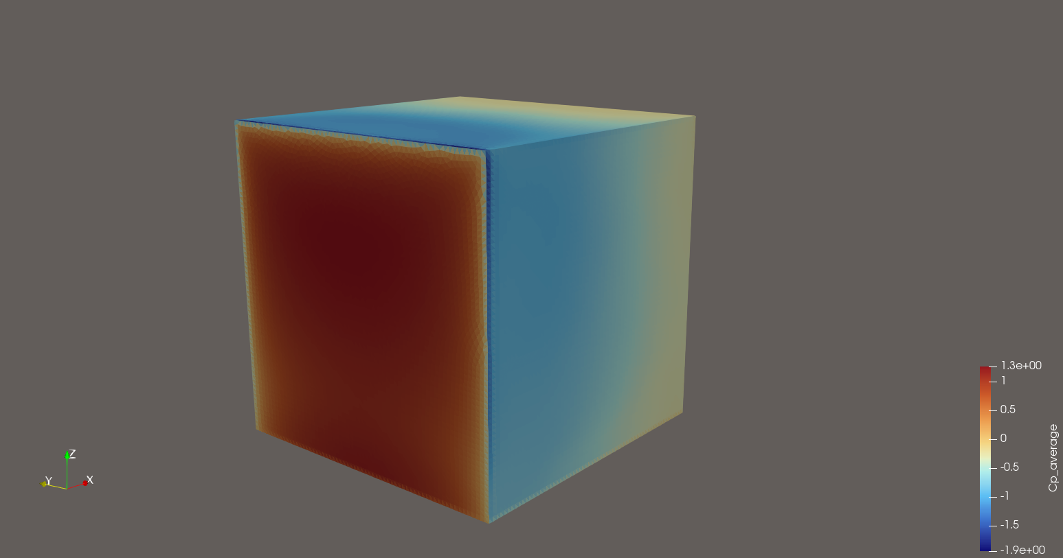
../../_images/03-cp-paraview.png — Pressure coefficient \(c_p\) visualised in ParaView on the body surface after running the script.¶