Setting Up the ABL Case
This guide walks through the complete configuration of a neutral Atmospheric Boundary Layer (ABL) simulation in AeroSim - from geometry import and domain sizing to mesh refinement, boundary conditions, solver settings, and export configuration. The goal is to generate and validate a turbulent ABL profile that matches a target terrain category and reference wind speed, which can then serve as an inlet condition or validation reference for building and urban studies.
Geometries
The first step is to import the geometries. This case uses two types:
Ground - a flat terrain surface that defines the no-slip floor of the domain
Roughness elements for the target terrain category: CAT I, CAT II, CAT III, CAT IV (CAT 0 - open sea - requires no roughness elements)
Roughness elements are arrays of solid fins distributed across the domain floor. They generate and sustain the turbulent shear layer by acting as physical obstacles that shed eddies at the correct scale. Each fin is 6 m wide, spaced on a 16 m × 32 m grid. Fin height is calibrated per terrain category according to EN 1991-1-4:
Terrain Category |
Description |
\(z_0\) (m) |
Fin height |
|---|---|---|---|
0 (sea) |
Open sea |
0.003 |
no fins |
I |
Open terrain with scattered obstacles |
0.01 |
\(1\,\text{m}\) |
II |
Open country with scattered obstacles |
0.05 |
\(2\,\text{m}\) |
III |
Suburban or industrial areas |
0.3 |
\(5\,\text{m}\) |
IV |
Dense urban centres |
1.0 |
\(7\,\text{m}\) |
This case uses terrain category II (\(z_0\) = 0.05 m). After importing the geometries, create a simulation named CAT2 and assign the ground surface and the CAT II roughness elements to it.
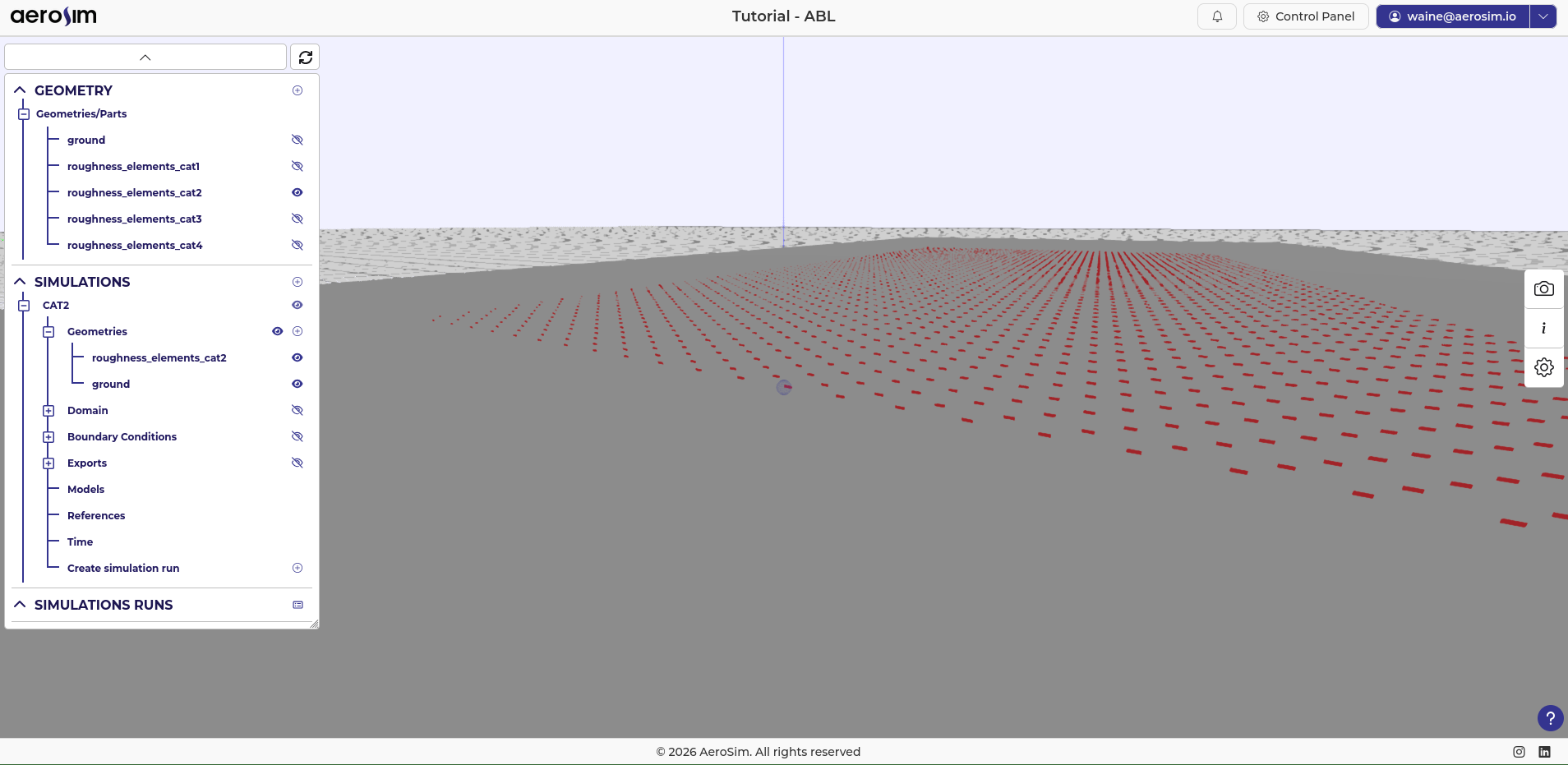
Imported geometries in the project tree after adding ground and CAT II roughness elements.
Domain Guidelines
AeroSim’s LBM solver achieves a memory efficiency of roughly 10 M nodes/GB, which makes large domains practical without a proportionally large GPU memory requirement. This case uses:
7200 m along wind (x) - minimum recommended is 6000 m
2000 m cross wind (y) - recommended at least \(2\times\) the width of the region of interest, and at least 1200 m
1000 m height (z) - recommended at least \(10\times\) the building height, and at least 800 m
Keep the blockage ratio - the fraction of the domain cross-section occupied by any geometry - below 5% in y and z.
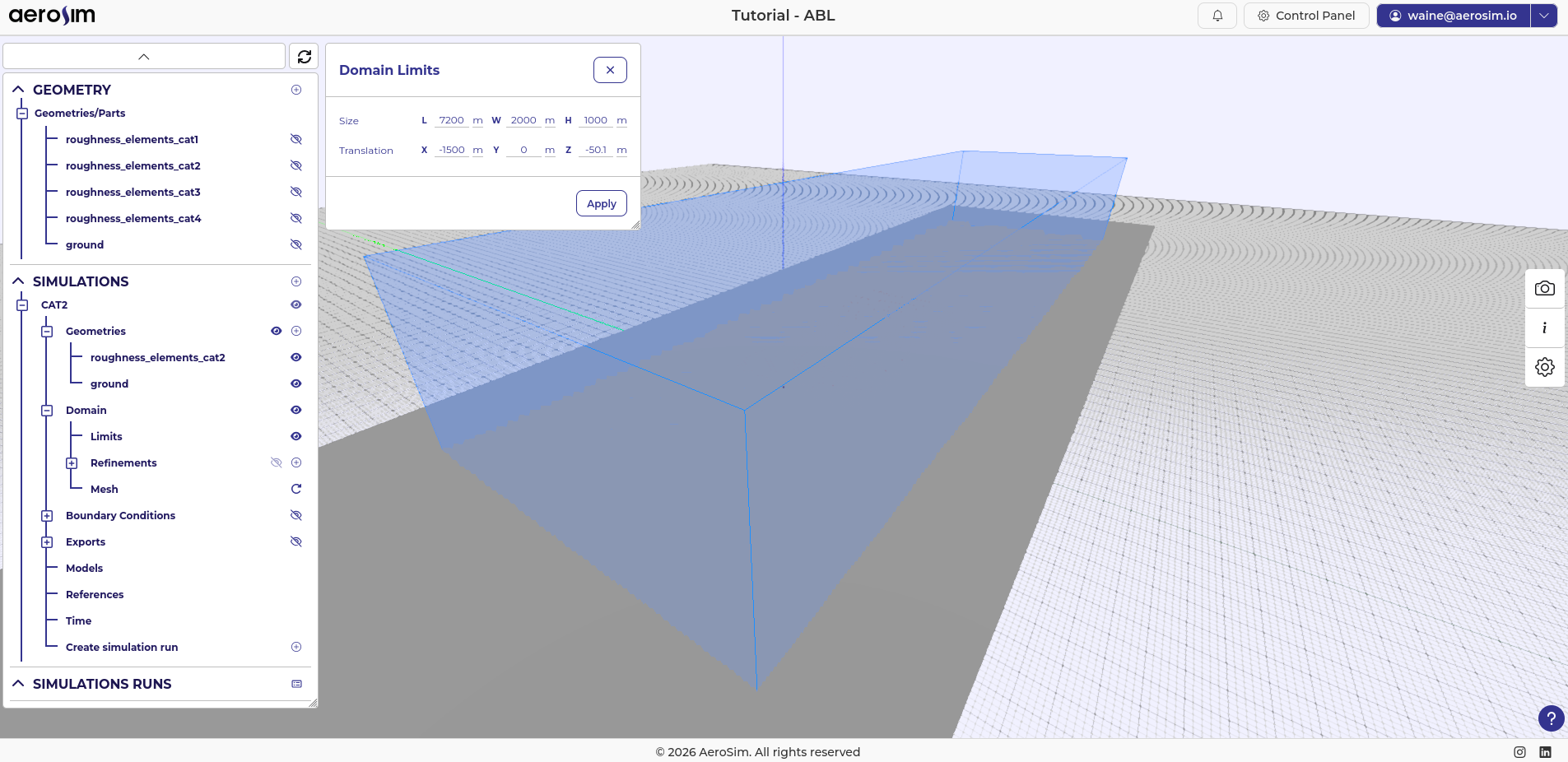
Initial domain geometry.
The domain is translated in x to place the region of interest at x = 0. A development length of 1500 m is used (recommended range is 1300 m to 1800 m), so the domain inlet sits at x = -1500 m. A small vertical offset of -50.1 m in z is also applied to prevent the domain boundary from coinciding with the ground geometry mesh, which avoids numerical issues at that interface.
Note
The development length allows the turbulent energy cascade to establish itself downstream of the inlet. Since SEM produces a synthetic profile, the flow needs a finite fetch to reorganise into a physically consistent state. This is most visible in the streamwise energy spectrum: examining how well the \(-5/3\) inertial subrange is recovered at \(x = 0\) is a good check that the development length is sufficient.
After the translation, the roughness elements should end at x = 0 (the start of the region of interest). Translate them -2000 m in x so their downstream face is aligned with that position.
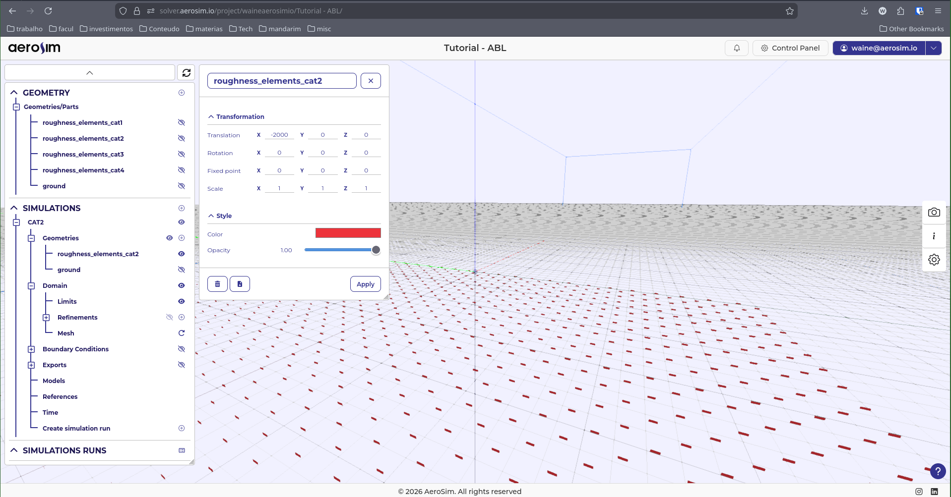
Roughness elements translated to end at the region of interest.
For the baseline resolution, use 10 m. This typically varies from 9 m to 12 m, balancing refinement level, memory usage, and runtime. At 10 m baseline, this mesh contains approximately 15 M nodes (~1.61 GB) - a relatively small mesh for AeroSim. Refinements added in the next section will increase this substantially.
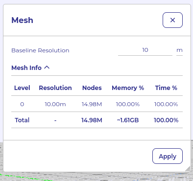
Initial mesh at \(10\,\text{m}\) baseline resolution (\({\sim}15\,\text{M}\) nodes).
Refinement Guidelines
After the domain is set up, box refinements are added to resolve the ABL near the ground. The target near-ground resolution for this case is 1.5 m (max 2.0 m), which is within the typical range of 1.2 m to 1.8 m.
Note
AeroSim uses octree refinement: each refinement level halves the cell size (strict 2:1 ratio). Starting from the 10 m baseline, three levels give the following progression:
Level |
Cell size |
|---|---|
Baseline |
\(10\,\text{m}\) |
Level 1 |
\(5\,\text{m}\) |
Level 2 |
\(2.5\,\text{m}\) |
Level 3 |
\(1.25\,\text{m}\) |
The target refinement controls the cell size AeroSim tries to achieve inside a refinement box; the max refinement caps the cell size at the box boundary. Setting both together controls how gradually the mesh transitions between levels.
Three refinement boxes are used:
ABL base spans from the domain inlet to 500 m downstream of the region of interest, with cross-wind extent ±100 m (y) and height 80 m (z). Target 1.5 m, max 2.0 m. Extents: (-1500, -100, -1) to (500, 100, 80)
Note
As a rule of thumb, height should be at least \(1.1\times\) the building height and cross-wind extent at least \(1\times\) the building width per side.
ABL transition 3 m surrounds the ABL base with a margin of \(\approx 50\times\) target resolution in x+ and \(\approx 20\times\) in y and z+. Target 3 m, max 4 m. Extents: (-1500, -160, -1) to (650, 160, 140).
ABL transition 6 m adds a further outer ring with proportional margins roughly doubling those of the inner ring. Target 6 m, max 8 m. Extents: (-1500, -280, -1) to (950, 280, 260).
Note
The margin values are rounded guidelines, not exact multiplications. There is no need to hit precise numbers - use values that are convenient to enter and result in a clean box layout.
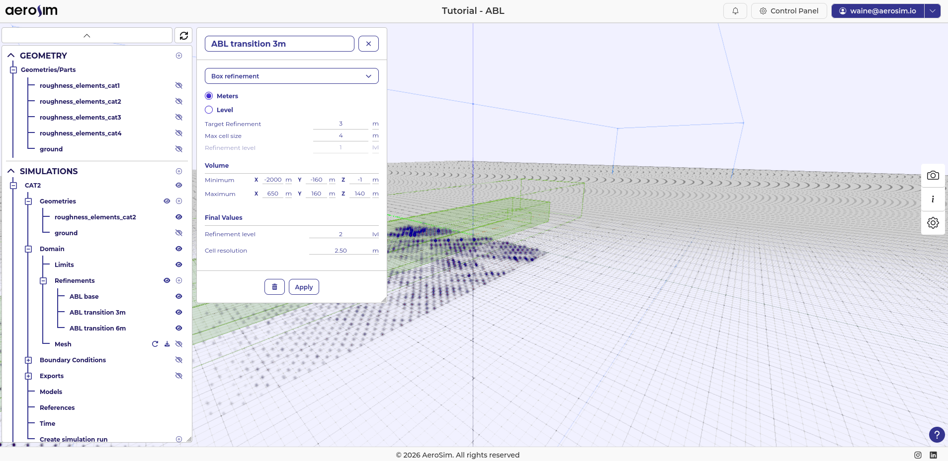
Final refinement configuration: ABL base, ABL transition \(3\,\text{m}\), and ABL transition \(6\,\text{m}\) boxes.
This yields a final mesh of approximately 47 M nodes, using about 5 GB of GPU memory.
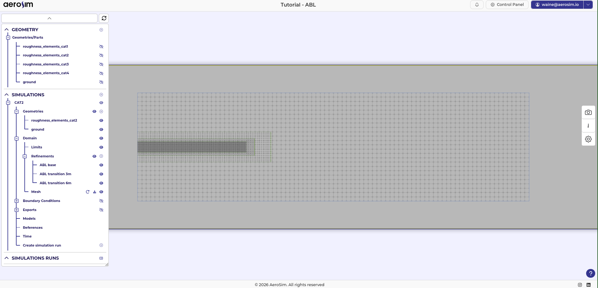
Final mesh after all refinement boxes (\({\sim}47\,\text{M}\) nodes, \({\sim}5\,\text{GB}\) GPU memory).
Note
To reduce node count, increase the baseline resolution. A 12 m baseline gives ~29 M nodes while still achieving a near-ground resolution of 1.5 m - a good trade-off for hardware with less GPU memory.
Boundary Conditions
Inlet
AeroSim uses the Synthetic Eddy Method (SEM) to generate physically consistent turbulent inflow. Rather than imposing a frozen smooth profile at the inlet face, SEM injects stochastic synthetic eddies superimposed on a prescribed mean velocity profile. The method ensures that the correct first- and second-order turbulent statistics - mean velocity and the full Reynolds stress tensor - are reproduced at the inlet plane.
AeroSim includes an automatic inlet profile generator (labelled ABL Equation in the interface). Given the terrain category and reference wind speed, it constructs the mean velocity and Reynolds stress profiles from standard analytical models, ready for direct use with the SEM inlet.
For this case the reference wind speed is \(U_{ref}\) = 20 m/s at \(z_{ref}\) = 10 m, and terrain category II (\(z_0\) = 0.05 m).
To configure the inlet:
Select the inlet face boundary condition and set the type to SEM.
For the profile source, choose From generator.
Enter Roughness length = 0.05 m, Target Velocity = 20 m/s, and Reference height = 10 m.
Click Apply.
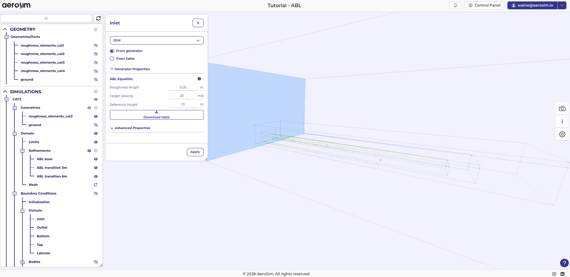
Inlet boundary condition configured as SEM with the ABL Equation profile generator.
Ground
The ground surface is set as Wall - ABL Wall Model with a roughness length of 0.05 m (matching the inlet profile for terrain category II).
The roughness elements imported earlier generate turbulence physically: the solid fins act as obstacles that shed eddies and sustain the turbulent boundary layer along the fetch. All solid surfaces - the ground and the fins - are treated via the Immersed Boundary Method (IBM). For the ABL Wall Model, it applies an equilibrium logarithmic law in near-wall cells using the local roughness length \(z_0\), removing the need to resolve the viscous sublayer.
This combination is AeroSim’s equivalent of the roughness-length boundary condition in OpenFOAM’s atm*WallFunction, operating natively within the LBM framework.
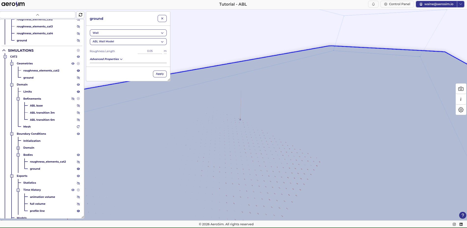
Ground body boundary condition set to Wall - ABL Wall Model with \(z_0 = 0.05\,\text{m}\).
Domain Faces
Top and lateral faces use Neumann conditions. These boundaries impose zero normal velocity gradient and zero shear stress, allowing the flow to pass through without introducing spurious wall effects. This is the standard choice for external aerodynamics when the domain is large enough that the boundary is outside the region of interest.
Outlet face uses a Neumann condition with fixed 0 pressure, which lets the flow exit freely while reducing the reflection of pressure waves back upstream.
Bottom face uses a no-slip condition, serving as a wall below the ground geometry.
These conditions are consistent with ABL simulations in OpenFOAM (slip at top/lateral, zeroGradient at outlet) and require no tuning for the ABL case.
Initialization
Set the initial flow field to a uniform velocity of 20 m/s in x. Starting from the reference velocity rather than from rest reduces the time the solver needs to reach a developed state, and is the standard initialisation for external aerodynamics cases.
Models
For the turbulence model, use LES with the Smagorinsky model and a Smagorinsky constant of 0.17.
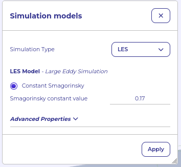
Models panel with LES Smagorinsky selected.
Reference Values
For the fluid density, use the standard air value \(\rho\) = 1.225 kg/m^3.
For the dynamic viscosity, AeroSim does not require the physical air value. Instead, it is chosen to target a specific Reynolds number. ABL flows operate at extremely high Reynolds numbers (\(Re \sim 10^8\) at full scale) that cannot be simulated directly; the standard practice in LES is to select a moderate \(Re\) that keeps the flow in the fully turbulent regime while making viscous effects negligible at the scales resolved by the mesh. A value of \(Re = 10^5\) is a suitable choice for most ABL cases.
With \(U_{ref} = 20\,\text{m/s}\), \(L_{ref} = 10\,\text{m}\), and \(Re = 10^5\):
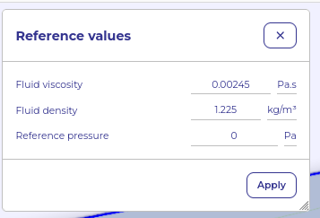
Reference values panel with fluid properties configured.
Time
Simulate for 720 s: the first 120 s serve as flow development and are discarded, and the remaining 600 s are used for statistics acquisition. The time step is \(\Delta t = 0.032\,\text{s}\), giving a CFL of 0.1. The estimated runtime shown by the interface is approximately 1h40min.
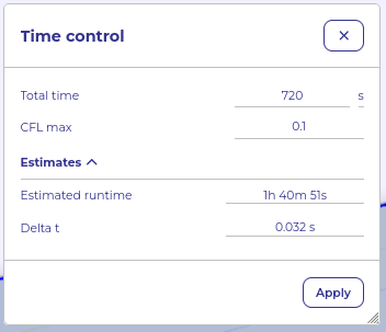
Time control panel with \(720\,\text{s}\) total simulation time and \(\Delta t = 0.032\,\text{s}\).
Note
CFL and LBM stability. The LBM operates in a weakly compressible regime where numerical stability requires the lattice Mach number \(Ma = U / (c_s \sqrt{3})\) to remain small. A CFL of 0.1 typically corresponds to \(Ma < 0.1\), keeping compressibility errors and numerical instabilities negligible. Exceeding \(Ma \approx 0.15\)-\(0.2\) risks numerical blow-up. This is why AeroSim recommends keeping the CFL at or below 0.1 for most cases.
Exports
Configure the exports before starting the run. This case uses four export items.
Statistics. A box spanning (-500, -200, 0) to (1000, 200, 200) collects field averages over the region of interest. Set the sampling period to 0.1 s and the start time to t = 120 s. Select the fields: Pressure, Velocity Ux, Uy, Uz.
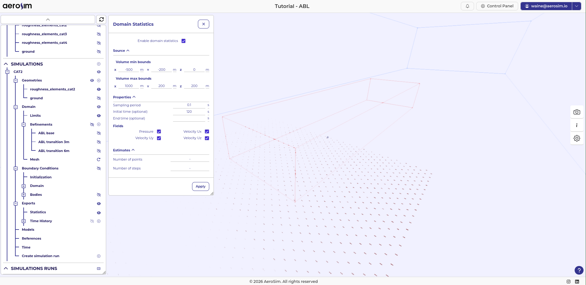
Statistics export: box around the region of interest, sampling every \(0.1\,\text{s}\) from \(t = 120\,\text{s}\).
Full volume (debug). A volume export from (-1500, -1000, -100) to (8000, 1000, 1000) covers the entire domain. Volumes may extend beyond the domain limits without issue. Use an export period of 100 s with no start or end time limit, and select all fields. This produces a few large snapshots useful for diagnosing the overall flow field without large storage overhead.
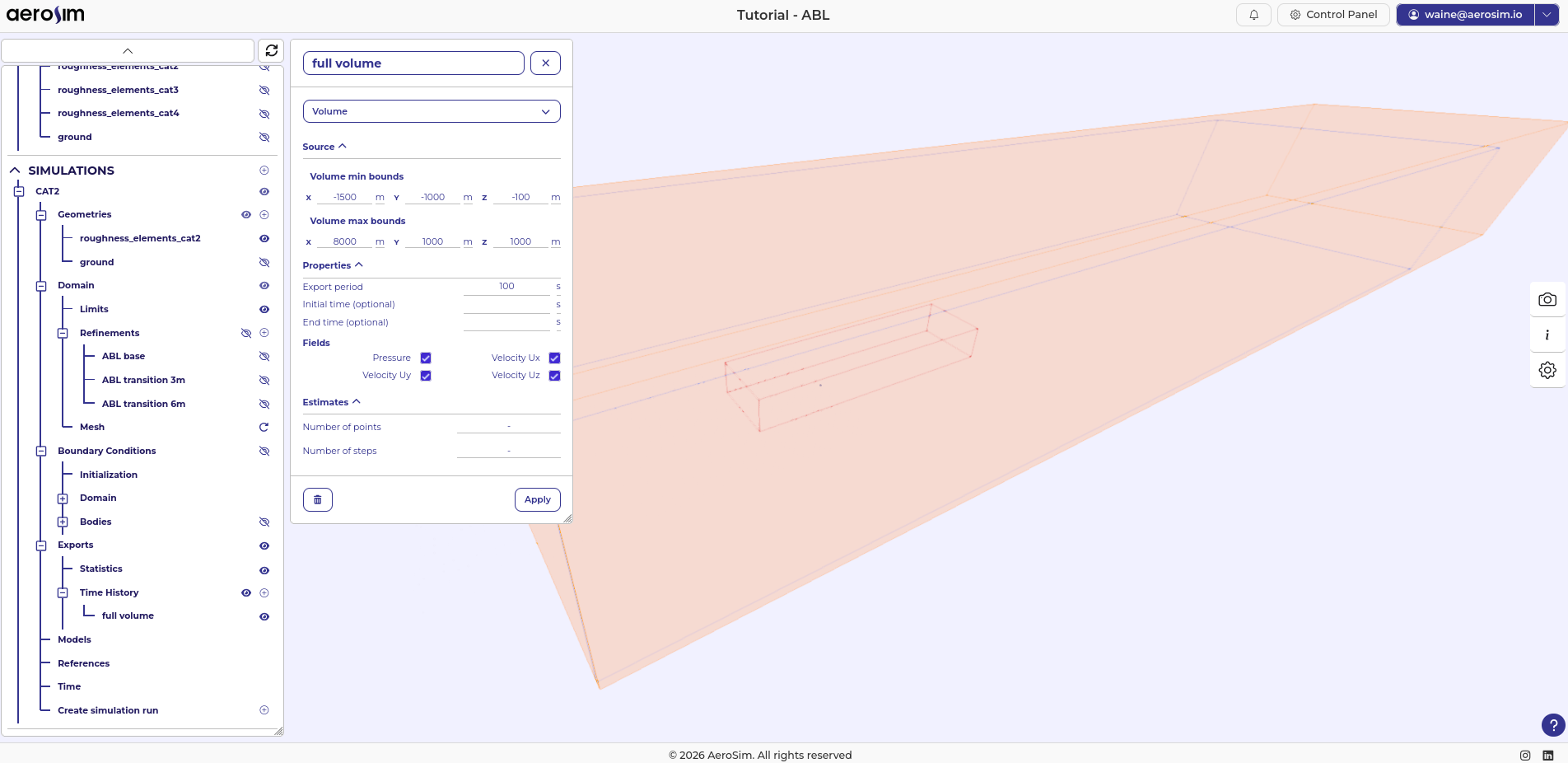
Full-volume export for domain-wide diagnostics.
Animation volume. A second volume export over the same box as the statistics export: (-500, -200, 0) to (1000, 200, 200). Set the sampling period to 0.1 s and limit the interval to t = 120 s to 140 s to keep file size manageable.
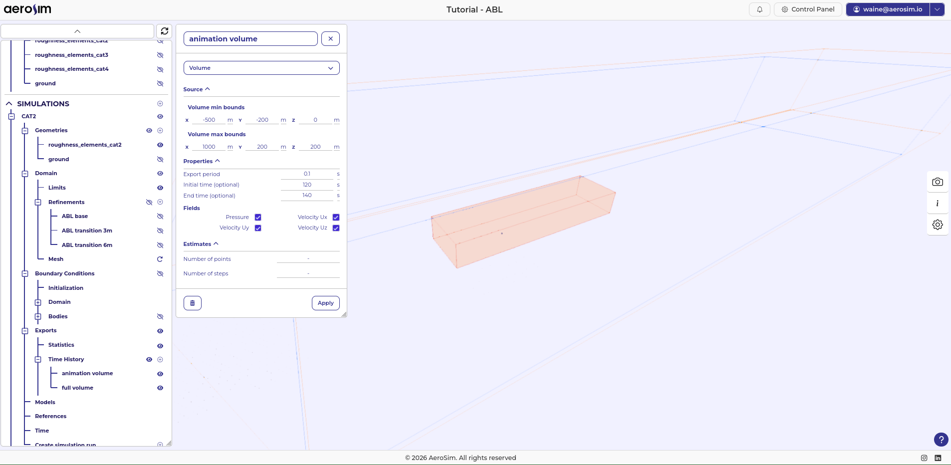
Animation export limited to \(t = 120\,\text{s}\)-\(140\,\text{s}\) to keep output size small.
Profile line. A vertical line from (0, 0, 0) to (0, 0, 200 m) with 201 points, sampled at 0.1 s from t = 120 s. Enable Velocity Ux, Uy, Uz (Pressure is not needed for profile analysis). The 0.1 s interval is short enough to resolve frequency spectra and turbulence intensity profiles, not just time-averaged statistics. Enable all export formats (XDMF, CSV, HDF) to cover downstream analysis needs.
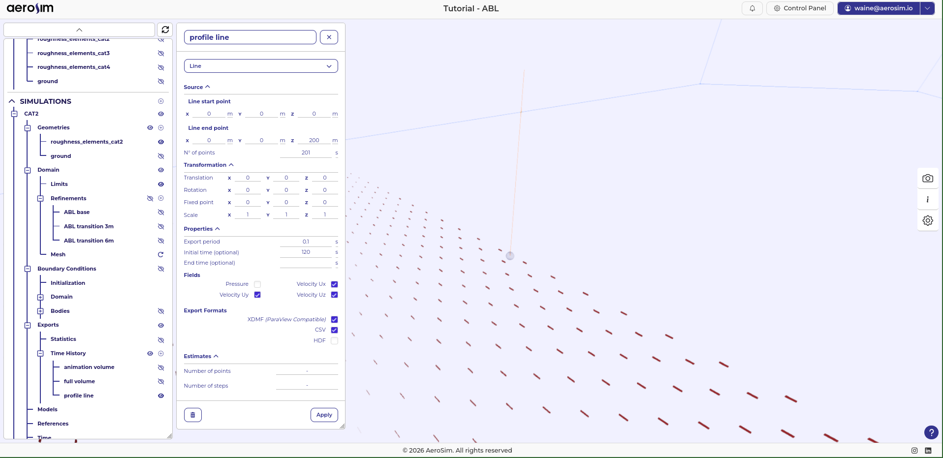
Vertical profile line at the origin (\(x = 0\), \(y = 0\)), sampled every \(0.1\,\text{s}\) from \(t = 120\,\text{s}\).
Next steps
With the simulation fully configured, run it. Once it completes, proceed to post-processing to analyse the velocity and turbulence intensity profiles and validate the generated ABL against the target terrain category.