Structural Load from Simulation¶

Wind-induced base shear force coefficients (\(C_{fx}\), \(C_{fy}\)) and the base torsional moment coefficient (\(C_{Mz}\)) are the primary inputs for the structural design of a building. Because they are dimensionless, they are independent of wind speed and can be combined with any design dynamic pressure to obtain the actual loads. This guide shows how to integrate the pressure coefficient \(c_p\) over the building surface to obtain time series of these coefficients.

Important

This workflow requires the \(c_p\) field to be already available in the body HDF5 file. Follow the Pressure Coefficient Measurement guide first to compute and store \(c_p\).

Definitions¶

Force Coefficient¶

The force coefficient is the dimensionless ratio between the net aerodynamic force and the product of dynamic pressure and a nominal area. Starting from the per-face force:

\[ \vec{F}_i(t) = -\,c_{p_i}(t)\;q\;A_i\;\hat{n}_i \]

the force coefficient in a given direction is obtained by summing over all \(N\) faces and normalising by the nominal area \(A_\text{nom}\):

\[ C_{fx}(t) = \frac{\sum_{i=1}^{N} F_{x_i}(t)}{q\,A_\text{nom}} = -\frac{\sum_{i=1}^{N} c_{p_i}(t)\;A_{i}\;\hat{n}_{x_i}}{A_\text{nom}} \]

The same applies for \(C_{fy}\). Note that the dynamic pressure \(q\) cancels out - the force coefficient depends only on \(c_p\) and the geometry.

Symbol	Quantity	Notes
\(c_{p_i}(t)\)	Pressure coefficient on face \(i\)	Time series from the previous step
\(A_i\)	Area of face \(i\)	Computed from the triangle vertices
\(\hat{n}_i\)	Outward unit normal of face \(i\)	Points away from the solid into the fluid
\(A_\text{nom}\)	Nominal (reference) area	User-defined; see below

The negative sign accounts for the convention that positive \(c_p\) means compression (pressure pushing into the surface), while the outward normal points away from it.

Moment Coefficient¶

The torsional moment coefficient \(C_{Mz}\) about a reference point \(O\) (typically the centroid of the building footprint at ground level) is normalised by the nominal volume \(V_\text{nom}\):

\[ C_{Mz}(t) = \frac{M_z(t)}{q\,V_\text{nom}} = -\frac{\sum_{i=1}^{N} \bigl( r_{x_i}\,c_{p_i}\,A_i\,\hat{n}_{y_i} - r_{y_i}\,c_{p_i}\,A_i\,\hat{n}_{x_i} \bigr)}{V_\text{nom}} \]

where \(\vec{r}_i = \vec{x}_{\text{centroid},i} - \vec{x}_O\) is the position vector from \(O\) to the centroid of face \(i\).

Note

The choice of reference point \(O\) affects the moment values. For structural design the standard choice is the geometric centre of the building footprint at ground level, because this is where the base reactions are evaluated. If you need moments about a different point (e.g. a floor slab), adjust the coordinates of \(O\) accordingly.

Nominal Area and Volume¶

The nominal area \(A_\text{nom}\) and nominal volume \(V_\text{nom}\) are user-defined reference quantities used for normalisation. For a rectangular building of width \(b\), depth \(d\), and height \(h\):

\[ A_\text{nom} = b \times h, \qquad V_\text{nom} = b \times d \times h \]

Computing Load Coefficients¶

The script below reads the body HDF5 file (which must already contain the cp/ group from the Pressure Coefficient Measurement step), extracts the mesh geometry from the XDMF descriptor, and integrates \(c_p\) over the building surface at every timestep to produce time series of \(C_{fx}\), \(C_{fy}\), and \(C_{Mz}\).

Prerequisites¶

Before running the script, make sure you have:

Run the compute_cp.py script from the Pressure Coefficient Measurement guide. The body HDF5 file must contain the cp/ group.
Both the HDF5 and XDMF files for the body surface export in the same directory.
Python packages: h5py and NumPy. Install them with pip install h5py numpy if not already available.

Parameters¶

Edit the top of the script to match your simulation:

Parameter	Description
`base_point`	Coordinates \((x, y, z)\) of the point about which the torsional moment is computed. Typically the centroid of the building footprint at ground level.
`nominal_area`	Reference area (m^2) for force coefficient normalisation.
`nominal_volume`	Reference volume (m^3) for moment coefficient normalisation.
`body_h5`	Path to the body HDF5 file (with the `cp/` group already written).
`body_xdmf`	Path to the body XDMF file (used to read mesh topology and vertex coordinates).

Script¶

Download compute_base_loads.py

import h5py
import numpy as np
import xml.etree.ElementTree as ET
from pathlib import Path

# ---------------------------------------------------------------
# Parameters - edit these to match your simulation
# ---------------------------------------------------------------

# Base point - the point about which the torsional moment is computed.
# Typically the centroid of the building footprint at ground level.
base_point = np.array([0.0, 0.0, 0.0])  # (x, y, z) in metres

# Nominal area and volume for normalisation.
# For a rectangular building of width b, depth d, and height h:
#   nominal_area   = b * h
#   nominal_volume = b * d * h
# Example for a building of 40x40x160
nominal_area   = 40*160     # m^2
nominal_volume = 40*40*160  # m^3

# File paths - adjust to the location of your downloaded files
base = Path(".")
body_h5   = base / "bodies.body_Cp body.h5"
body_xdmf = base / "bodies.body_Cp body.xdmf"
output_csv = base / "base_load_coefficients.csv"
# ---------------------------------------------------------------


# ----- Step 1: read mesh from XDMF / HDF5 -----
print("Reading mesh geometry from XDMF ...")
tree = ET.parse(body_xdmf)
root = tree.getroot()
domain = root.find("Domain")
collection = domain.find("Grid")
first_grid = collection.findall("Grid")[0]

# Topology (triangle connectivity)
topo_elem = first_grid.find("Topology")
topo_data = topo_elem.find("DataItem")
topo_ref = topo_data.text.strip()  # e.g. "file.h5:/path"
topo_h5_file, topo_h5_path = topo_ref.split(":")

# Geometry (vertex coordinates)
geom_elem = first_grid.find("Geometry")
geom_data = geom_elem.find("DataItem")
geom_ref = geom_data.text.strip()
geom_h5_file, geom_h5_path = geom_ref.split(":")

# Resolve HDF5 paths relative to the XDMF directory
xdmf_dir = body_xdmf.parent
topo_h5_path_full = xdmf_dir / topo_h5_file
geom_h5_path_full = xdmf_dir / geom_h5_file

with h5py.File(topo_h5_path_full, "r") as f:
    triangles = f[topo_h5_path][:]  # (N_tri, 3) - vertex indices

with h5py.File(geom_h5_path_full, "r") as f:
    vertices = f[geom_h5_path][:]  # (N_vert, 3) - xyz coordinates


# ----- Step 2: compute face normals, areas, and centroids -----
print("Computing face normals, areas, and centroids ...")
v0 = vertices[triangles[:, 0]]
v1 = vertices[triangles[:, 1]]
v2 = vertices[triangles[:, 2]]

edge1 = v1 - v0
edge2 = v2 - v0
cross = np.cross(edge1, edge2)  # (N_tri, 3)

# Area = 0.5 * |cross product|
area = 0.5 * np.linalg.norm(cross, axis=1)  # (N_tri,)

# Unit outward normal
normals = cross / (2.0 * area[:, np.newaxis])  # (N_tri, 3)

# Face centroid = mean of three vertices
centroids = (v0 + v1 + v2) / 3.0  # (N_tri, 3)

# Area-weighted normal vectors (A_i * n_hat_i)
area_normals = area[:, np.newaxis] * normals  # (N_tri, 3)

# Lever arm from base point to each face centroid
lever_arm = centroids - base_point[np.newaxis, :]  # (N_tri, 3)

n_tri = len(triangles)
print(f"  {n_tri} triangles")
print(f"  Nominal area   = {nominal_area} m^2")
print(f"  Nominal volume = {nominal_volume} m^3")


# ----- Step 3: read Cp and integrate force / moment coefficients -----
print("Reading Cp and integrating load coefficients ...")
with h5py.File(body_h5, "r") as f:
    if "cp" not in f:
        raise RuntimeError(
            "No 'cp' group found in the body HDF5 file. "
            "Run compute_cp.py first to add pressure coefficients."
        )
    cp_keys = sorted(f["cp"].keys(), key=lambda k: float(k[1:]))
    n_steps = len(cp_keys)

    # Pre-allocate output arrays
    times = np.empty(n_steps)
    Cfx = np.empty(n_steps)
    Cfy = np.empty(n_steps)
    CMz = np.empty(n_steps)

    for i, key in enumerate(cp_keys):
        cp = f[f"cp/{key}"][:]  # (N_tri,)
        times[i] = float(key[1:])  # strip the leading 't'

        # Force coefficient per face: cf_i = -cp_i * A_i * n_hat_i / A_nom
        # The negative sign accounts for pressure acting inward
        # on the surface (positive cp = compression = inward force).
        # Summing over all faces gives the global force coefficient.
        Cfx[i] = -(cp * area_normals[:, 0]).sum() / nominal_area
        Cfy[i] = -(cp * area_normals[:, 1]).sum() / nominal_area

        # Torsional moment coefficient:
        # CMz = sum( rx * cfy_i - ry * cfx_i ) / V_nom
        fx_per_face = -cp * area_normals[:, 0]
        fy_per_face = -cp * area_normals[:, 1]
        CMz[i] = (
            lever_arm[:, 0] * fy_per_face
            - lever_arm[:, 1] * fx_per_face
        ).sum() / nominal_volume

        if (i + 1) % 100 == 0 or (i + 1) == n_steps:
            print(f"  {i + 1}/{n_steps} timesteps", end="\r")

print(f"\nIntegrated {n_steps} timesteps over {n_tri} faces.")


# ----- Step 4: write results to CSV -----
print(f"Writing results to {output_csv} ...")
header = "time,Cfx,Cfy,CMz"
data = np.column_stack([times, Cfx, Cfy, CMz])
np.savetxt(output_csv, data, delimiter=",", header=header, comments="",
           fmt="%.6e")

print("Done.")
print(f"  Cfx range: [{Cfx.min():.4f}, {Cfx.max():.4f}]")
print(f"  Cfy range: [{Cfy.min():.4f}, {Cfy.max():.4f}]")
print(f"  CMz range: [{CMz.min():.4f}, {CMz.max():.4f}]")

Output¶

The script writes a CSV file (base_load_coefficients.csv) with the following columns:

Column	Description
`time`	Simulation time (s)
`Cfx`	Force coefficient in the \(x\)-direction (along-wind)
`Cfy`	Force coefficient in the \(y\)-direction (across-wind)
`CMz`	Torsional moment coefficient about the \(z\)-axis

Note

The same integration approach can be used to obtain the remaining components (\(C_{fz}\), \(C_{Mx}\), \(C_{My}\)) if needed. The script can be extended by summing the corresponding area-normal and cross-product components.

The CSV can be loaded into ParaView, a spreadsheet, or any plotting tool to visualise the time series alongside the building surface.

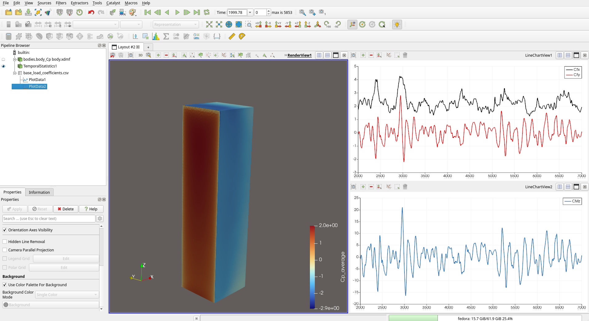
../../_images/01-load-coefficients-paraview.png — Load coefficient time series (\(C_{fx}\), \(C_{fy}\), \(C_{Mz}\)) plotted in ParaView alongside the building surface coloured by \(c_p\).¶

Interpreting the Results¶

Sign Convention¶

The sign of each component follows the right-hand rule applied to the simulation coordinate system. In a typical AeroSim setup where \(x\) is the along-wind direction:

\(C_{fx} > 0\): net force pushes the building in the \(+x\) (downwind) direction - this is the along-wind drag coefficient.
\(C_{fy}\): across-wind force coefficient, which oscillates around zero for a symmetric building in smooth flow but can have a nonzero mean under turbulent or asymmetric conditions.
\(C_{Mz}\): torsional moment coefficient about the vertical axis. A nonzero mean \(C_{Mz}\) indicates an asymmetric pressure distribution (e.g. from irregular building geometry or surrounding buildings).

Statistical Quantities¶

From the time series you can extract the standard statistics used in wind engineering:

Mean (\(\overline{C_f}\), \(\overline{C_M}\)): the time-averaged coefficient, used for static design checks.
Peak (\(\hat{C_f}\), \(\hat{C_M}\)): the maximum instantaneous coefficient, used for ultimate limit state checks.
RMS (\(\sigma_{C_f}\), \(\sigma_{C_M}\)): the standard deviation of the fluctuating component, used for fatigue and dynamic response assessments.

Obtaining Dimensional Loads¶

To convert the dimensionless coefficients into forces (N) and moments (N.m) for a specific design condition, multiply by the design dynamic pressure and the corresponding reference quantity:

\[ F_x = C_{fx}\;q_\text{design}\;A_\text{nom}, \qquad F_y = C_{fy}\;q_\text{design}\;A_\text{nom} \]

\[ M_z = C_{Mz}\;q_\text{design}\;V_\text{nom} \]

where the design dynamic pressure is:

\[ q_\text{design} = \tfrac{1}{2}\,\rho\,U_\text{design}^2 \]

This separation between the aerodynamic coefficient (from the simulation) and the design wind speed (from the wind code or site-specific study) is the standard practice in wind engineering. The same coefficient time series can be reused for different wind speed scenarios without rerunning the simulation.

Appendix: Geometric Quantities from the Mesh¶

The force and moment integrals require three geometric properties per triangle. The script computes them directly from the vertex coordinates stored in the XDMF/HDF5 files. This section documents the formulas for reference.

Face normal and area. For a triangle with vertices \(\vec{v}_0\), \(\vec{v}_1\), \(\vec{v}_2\):

\[ \vec{n}_i = (\vec{v}_1 - \vec{v}_0) \times (\vec{v}_2 - \vec{v}_0) \]

\[ A_i = \tfrac{1}{2}\,|\vec{n}_i|, \qquad \hat{n}_i = \frac{\vec{n}_i}{|\vec{n}_i|} \]

Face centroid. The centroid of the triangle is the arithmetic mean of its vertices:

\[ \vec{x}_{\text{centroid},i} = \frac{\vec{v}_0 + \vec{v}_1 + \vec{v}_2}{3} \]

Lever arm. The position vector from the base point to the face centroid:

\[ \vec{r}_i = \vec{x}_{\text{centroid},i} - \vec{x}_O \]

Tip

All these quantities are static - they depend only on the mesh and need to be computed once. Only the \(c_p\) time series changes at each timestep.