
 AeroSim Docs
4. Solver Numerics
For the solver setup, we will set the boundary conditions, the numerical models and the parameters for the simulation.
Boundary Conditions and Initialization
For the boundary conditions, the most important one we will set here is the inlet.
AeroSim uses SEM (synthetic eddy method) for its ABL inflow profile, combining the Eurocode velocity and turbulence intensity profiles with heuristics to achieve a “good enough” profile for the simulation inlet. It is important to note that this inflow still needs to develop into a physical flow through the domain, which is why the development length is used.
In SEM we set:
Profile -> Log Law
Roughness length -> the same as the category we are using (CAT 2), 0.05 m
Target velocity and reference height -> these can be chosen arbitrarily; for this case we set 5 m/s and 3 m
The profile can be seen after applying all changes and reloading it.
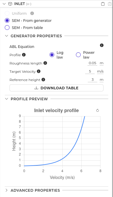
The SEM inlet form and the resulting inflow profile.
For the initialization we set SEM Field, which makes the velocity field start with the inlet average.
The other BCs are the defaults for ABL flows:
Outlet -> Fixed Pressure (0 Pa)
Laterals -> Neumann
Bottom -> Wall
Top -> Neumann
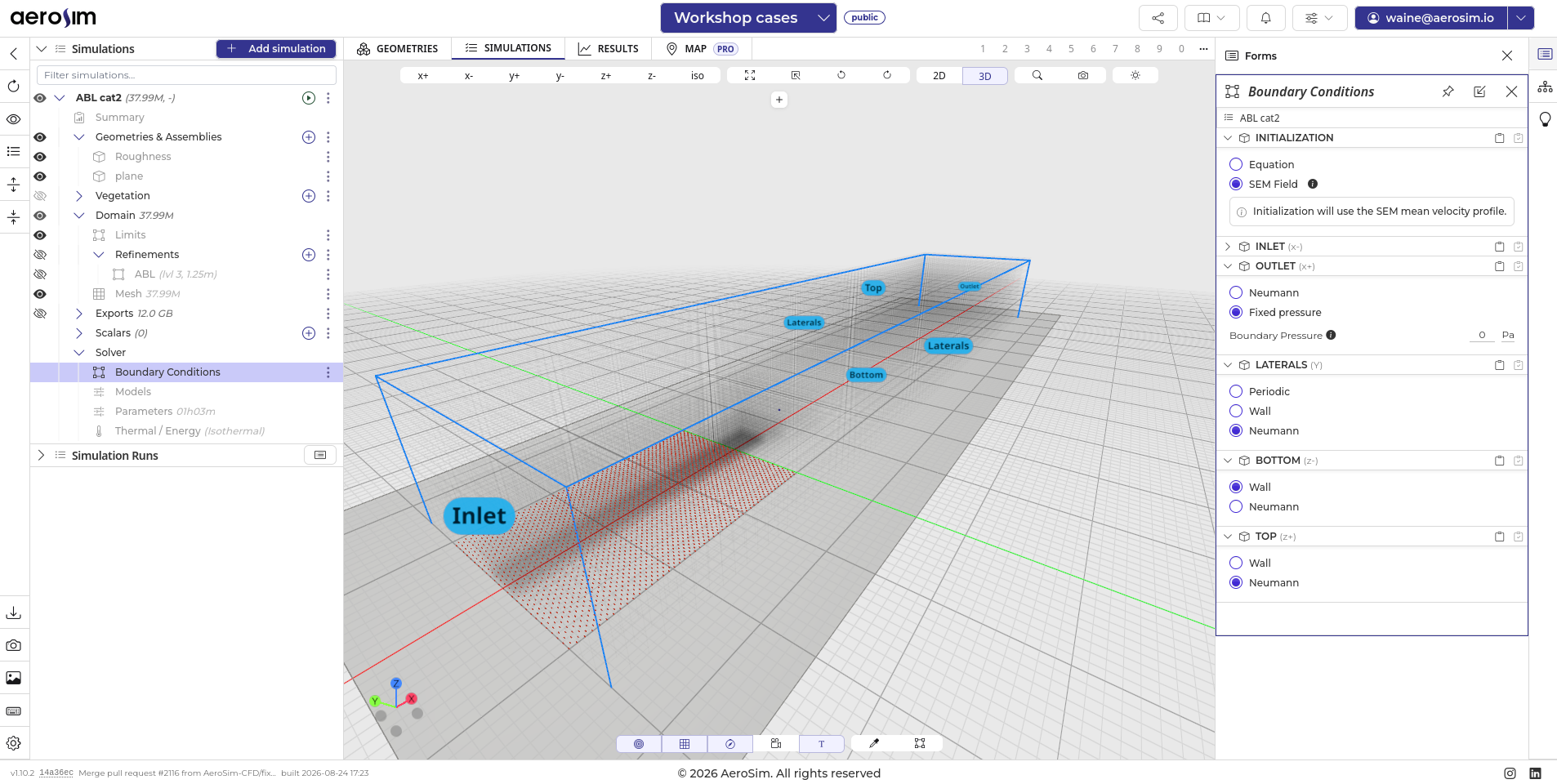
All boundary conditions set for the ABL case.
See also
Synthetic Eddy Method (SEM) explains what the inlet generates and how the parameters map to the target profile.
Models
For the models, we will use the default: LES Smagorinsky model with a Smagorinsky constant of 0.17.
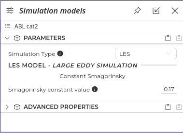
The numerical models form, with the default LES Smagorinsky setup.
Parameters
For the parameters, we choose the dynamic viscosity to match the Reynolds number. In this case, 0.0002 Pa s gives ~90k Re considering the velocity and reference height we set. For the fluid density we use the air value, ~1.225 kg/m^3.
For time, we recommend about 2 FTTs (flow through times) for development in negative time, considering the flow from the inlet to the position of interest, which is usually 0 m. One FTT here is 1500 m / 5 m/s = 300 s, so the simulation is set to start at -600 s.
For the acquisition time (after 0 s) we will use 1000 CTS (convective time scale) for this case, which is generous overall. The CTS is calculated by \(L/U\), using \(L = 3\,\text{m}\) and \(U = 5\,\text{m/s}\), which yields 0.6 s for this case. So the acquisition time will be 600 s.
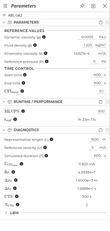
The parameters form, with viscosity, density and the simulation time window.
Most of these values can be calculated using the diagnostics inside the form and tweaked around it. Note that the diagnostics panel computes \(L/U\) from whatever representative length is entered there, so with 1500 m it reports the development scale (300 s, 2 of them) and not the 0.6 s body scale we used for the acquisition time. Both are convective time scales, on different lengths.
See also
Convective Time Scale and Simulation Timing covers the difference between the development and the statistics time scales, and how many of each a run actually needs.
With all that we can check the simulation time. The performance metric used by the AeroSim solver is MLUPS (million lattice updates per second). The default guessed value is 500, but simulations may get up to 1500 MLUPS depending on the setup and the GPU model.
The final expected time for this case is about 1h20 at the default 500 MLUPS, a common time for ABL cases in the AeroSim solver.
Next steps
Now we have set up most of our simulation, but before running it we must set its data exports.