3. Results

With the run finished, we download the exports and process the pressure on the building into pressure coefficients.

Downloading the results

The first thing to do is download the results we need: the body export and the point pressure, which are the two that feed the \(c_p\), plus some debug visualizations, such as the statistics field and the XZ plane.

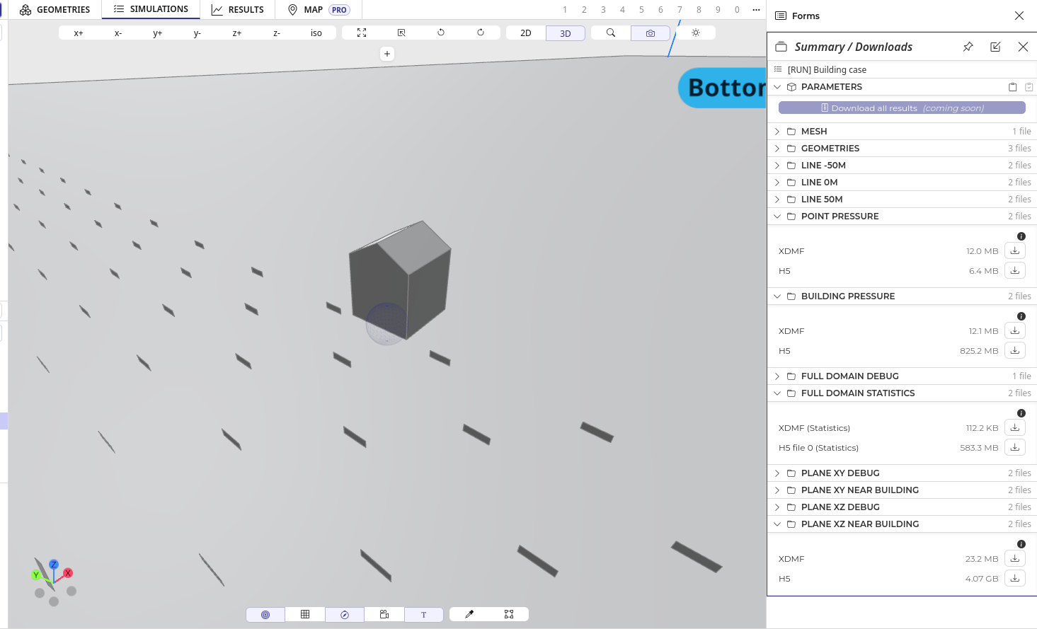
The downloads panel of the run, with the body export (building pressure) and the reference point among the available files.

Computing the pressure coefficient

The pressure coefficient is defined as

\[ c_p(t) = \frac{p(t) - p_\infty(t)}{\tfrac{1}{2}\rho U^2} \]

where \(\rho\) is the air density, \(p(t)\) the pressure at the body, \(p_\infty(t)\) the reference pressure and \(U\) the reference velocity.

Note

Both pressures are time series, and the subtraction has to be done point by point in time. The Pressure Coefficient Measurement guideline explains why a constant \(p_\infty\) distorts the result.

For the reference velocity we take the mean profile, either from the previous case or from a profile upstream of the building, at the building height of 25 m. Here we use the statistics field at -100 m, which gives about 7.75 m/s. The density is the one we set in the simulation setup, 1.225 kg/m^3.

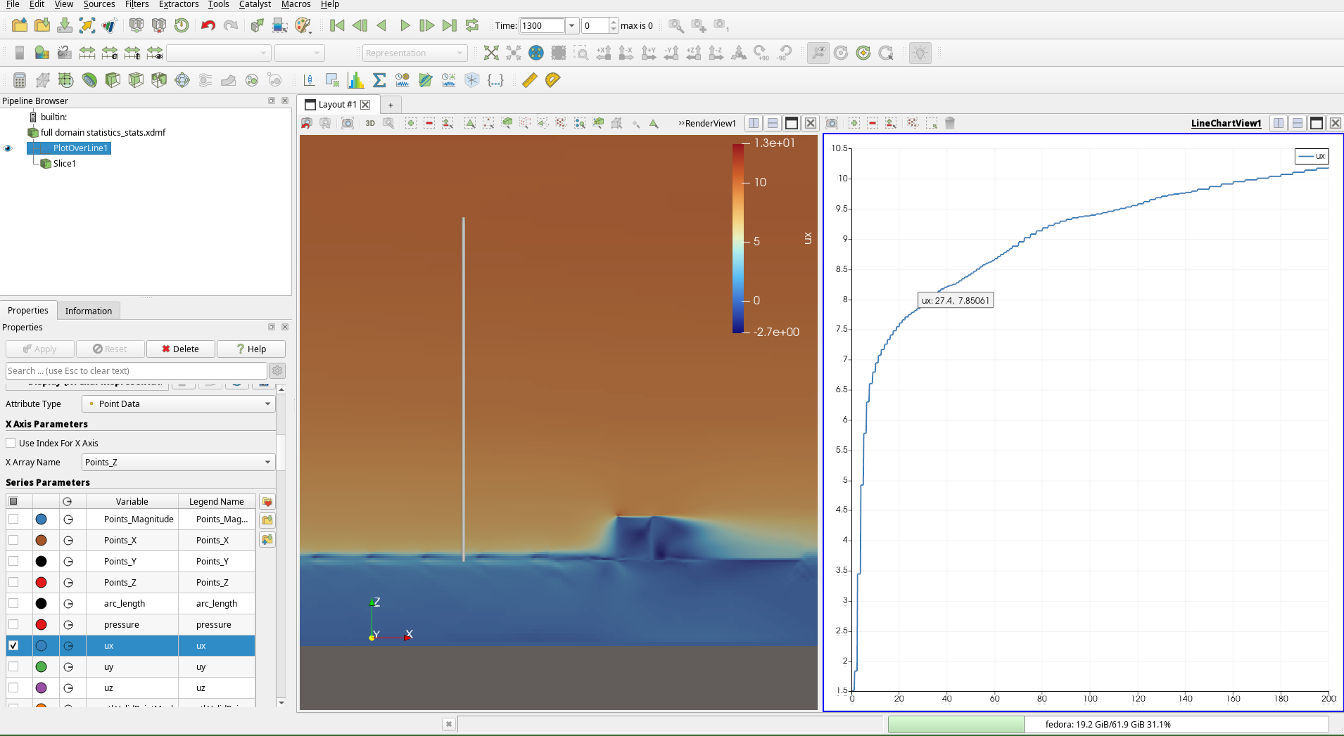
The mean streamwise velocity profile taken from the statistics field upstream of the building, with a Plot Over Line at \(x = -100\,\text{m}\).

With these values the dynamic pressure is 36.79 Pa, so the coefficient becomes \(c_p(t) = (p(t) - p_\infty(t)) / 36.79\).

To generate it, we recommend using the compute_cp.py script, which computes the coefficient and embeds it in the body file.

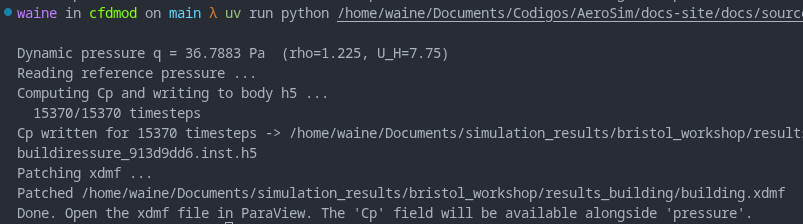
The script run, writing \(c_p\) for the 15370 exported timesteps into the body file and patching its XDMF.

Visualizing it

Now we just open the building file in ParaView, and both Cp and pressure should be present.

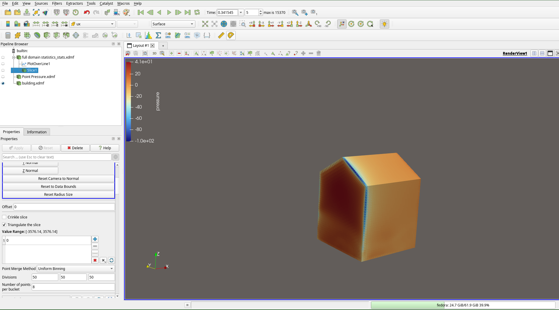
The body surface colored by the instantaneous pressure field.

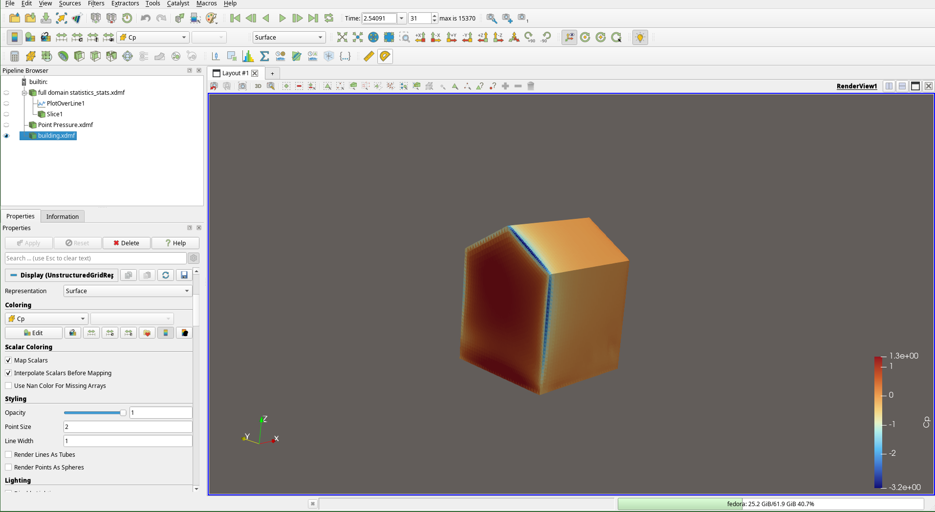
The same instant colored by Cp, now dimensionless.

From here it is possible to compute statistics, process forces on surfaces, export animations and other things with the pressure time series. The mean field, for example, comes from a Temporal Statistics filter over the body.

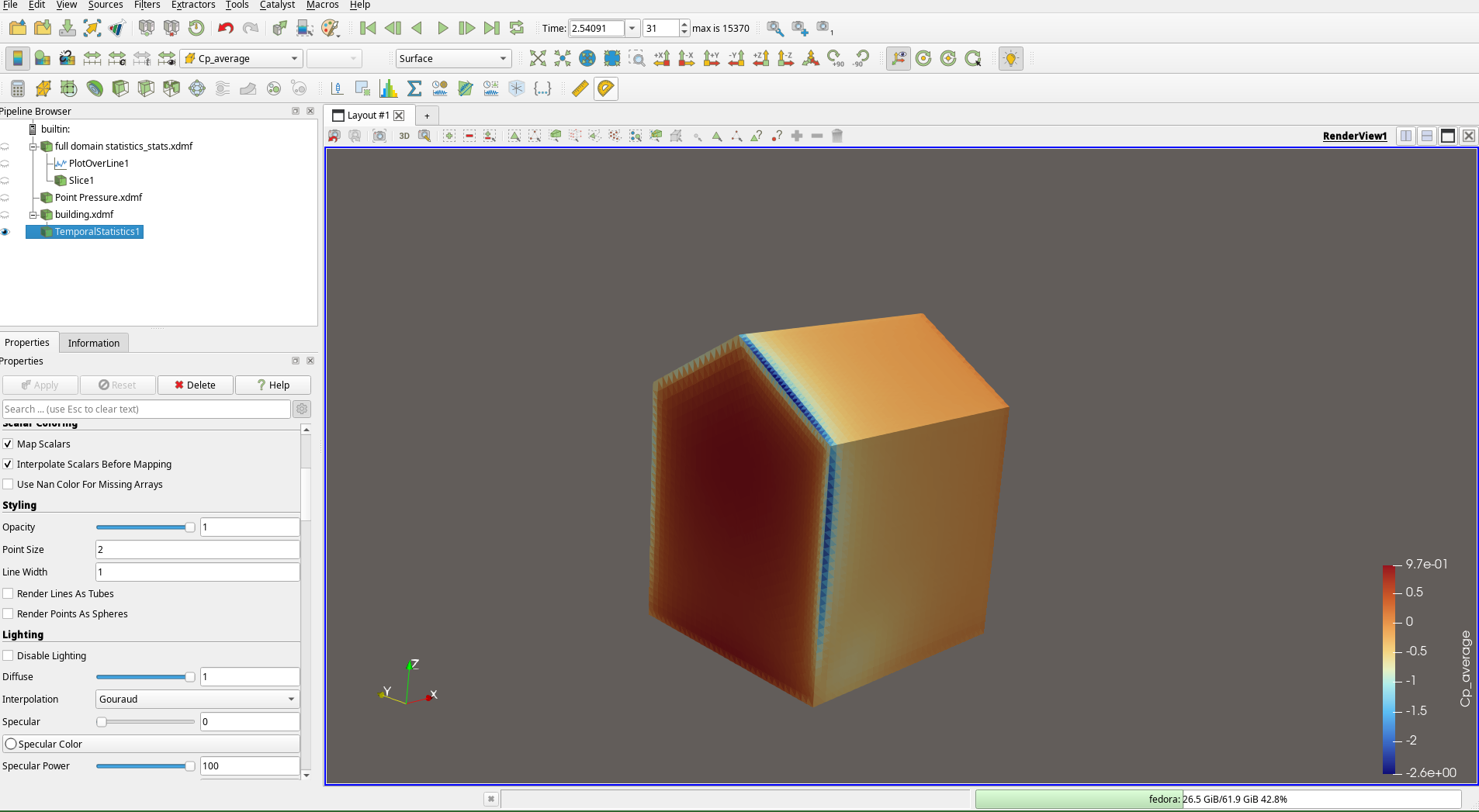
The mean pressure coefficient, Cp_average, from a Temporal Statistics filter over the whole acquisition window.

Animating the instantaneous field is also a good way to see the flow acting on the building, with the stagnation on the windward face and the fluctuating suction on the roof and on the side walls.

Instantaneous pressure coefficient on the building surface, animated over the acquisition window.

See also

Pressure Coefficient Measurement covers the \(c_p\) definition and ships the script used to compute it from these two exports.

Next steps

With the results processed, we can recap the whole path.