7. Results

Now that we have run the case, we must check the results. Previously we downloaded all the macroscopics from the case, and now we will visualize them in ParaView.

Note

The results shown in this chapter come from a slightly different setup, so you can expect different values and plots from the ones you get by following this workshop. The inspection is done the same way.

Processing the Lines

For lines, we can visualize them in the domain by adding the geometries as well, which makes it easier to check the positions.

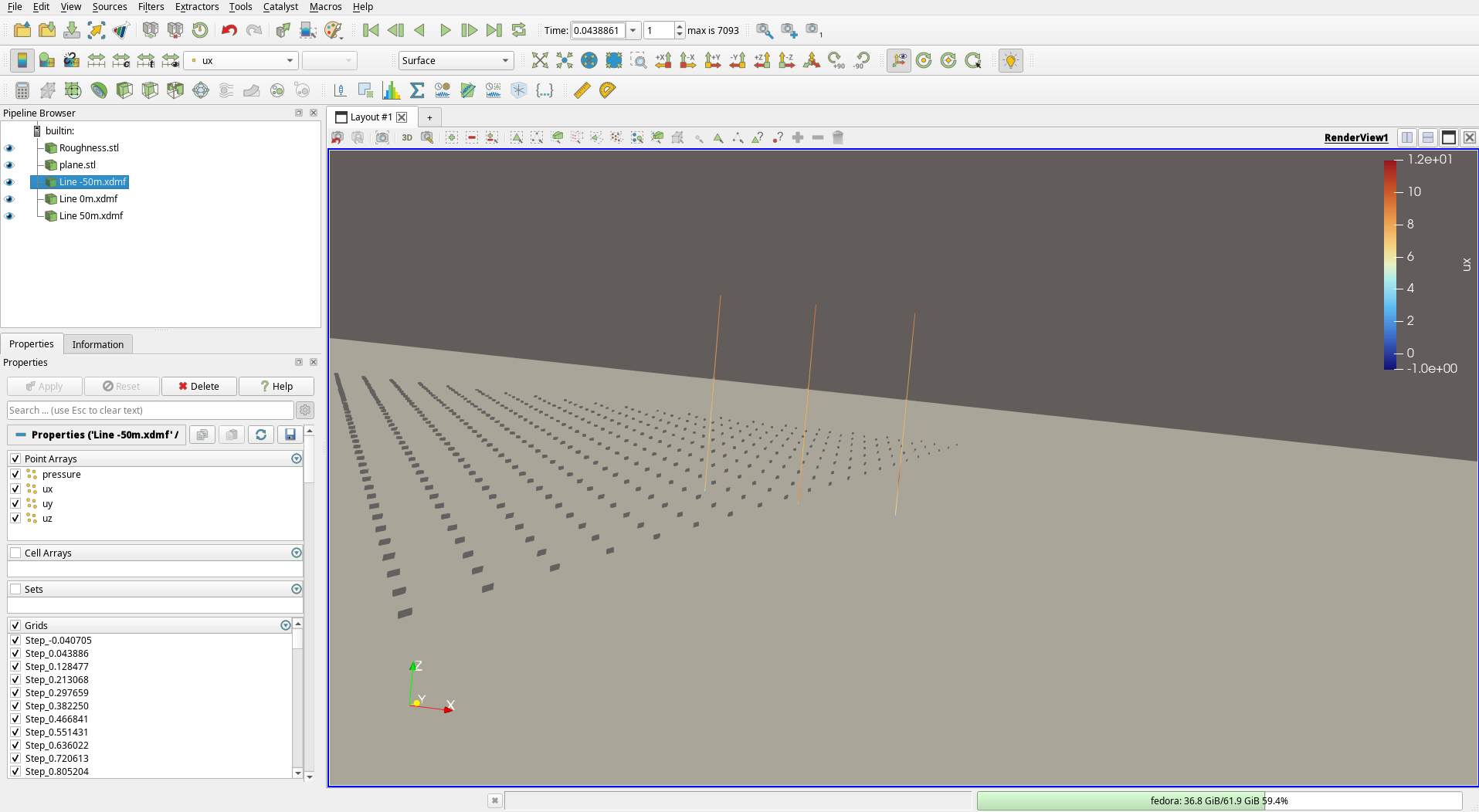
The three line exports loaded alongside the plane and roughness geometries, coloured by \(u_x\).

To process the average velocity in them and see how it changes, we add Temporal Statistics, and then Plot Data on the line, using the z position as x and ux as y.

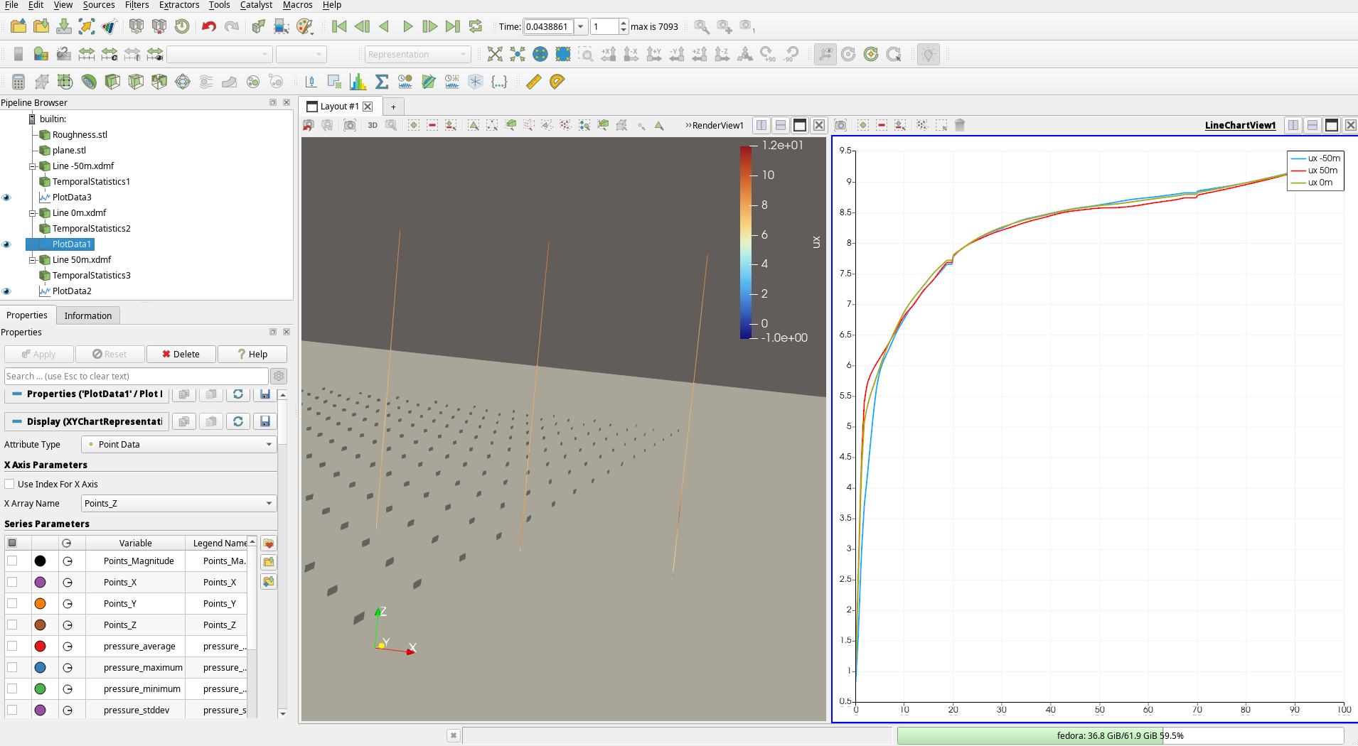
Mean \(u_x\) profiles for the three lines, plotted against Points_Z.

We can also add a turbulence intensity Calculator (ux_stddev/ux_average) on top of the temporal statistics and plot it.

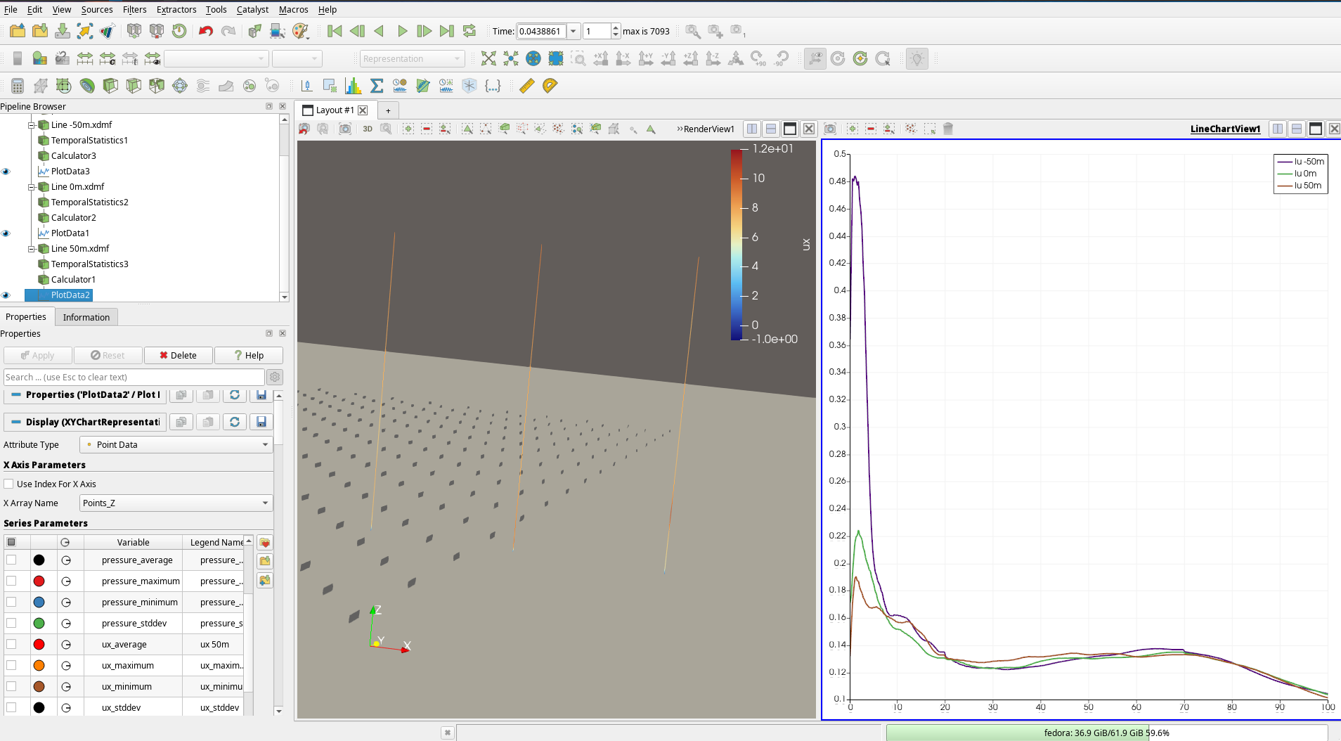
Turbulence intensity profiles for the three lines.

We compare the results against the Eurocode values using the script below. It reads the line exports directly from their HDF5 files and plots both profiles against EN 1991-1-4 for terrain category II.

Note

The script requires h5py, NumPy and Matplotlib. Run it from the folder holding the downloaded line exports: python plot_abl_eurocode.py --dir <results folder>.

Download plot_abl_eurocode.py

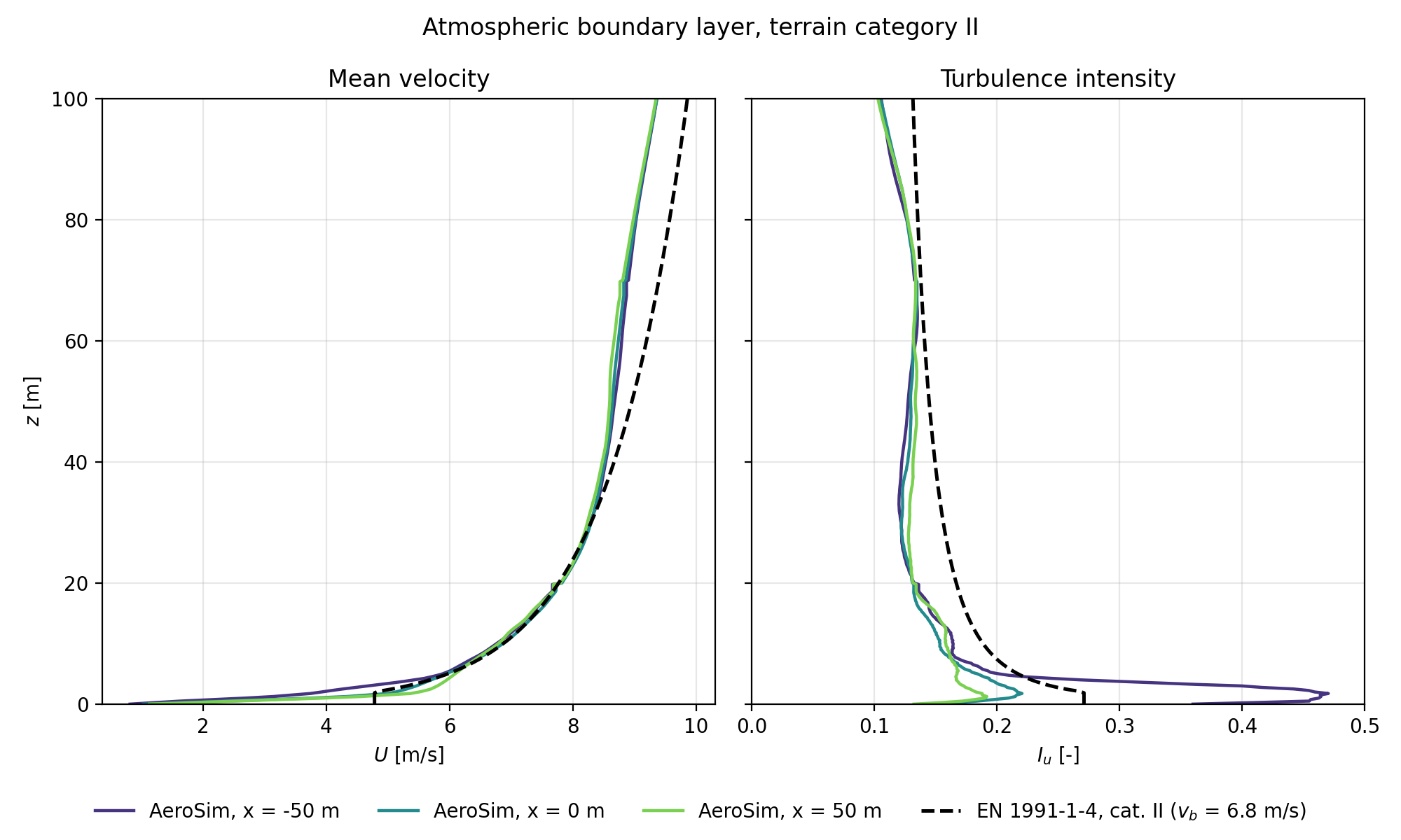
Mean velocity and turbulence intensity from the three lines, against EN 1991-1-4 terrain category II.

For the average velocity, the plot is pretty spot on. For the turbulence intensity, the values are lower than Eurocode CAT 2. To improve this we could go back to the setup and, for example, try to increase the elements height, increase the K multiplier in the advanced properties of SEM, increase the roughness category, or other tweaks. Even changing the resolution may affect this. It’s a process of trial and error.

Visualizing the Domain

For domain visualization we will use the XZ plane as an example: we open the XDMF file and just check its visualization.

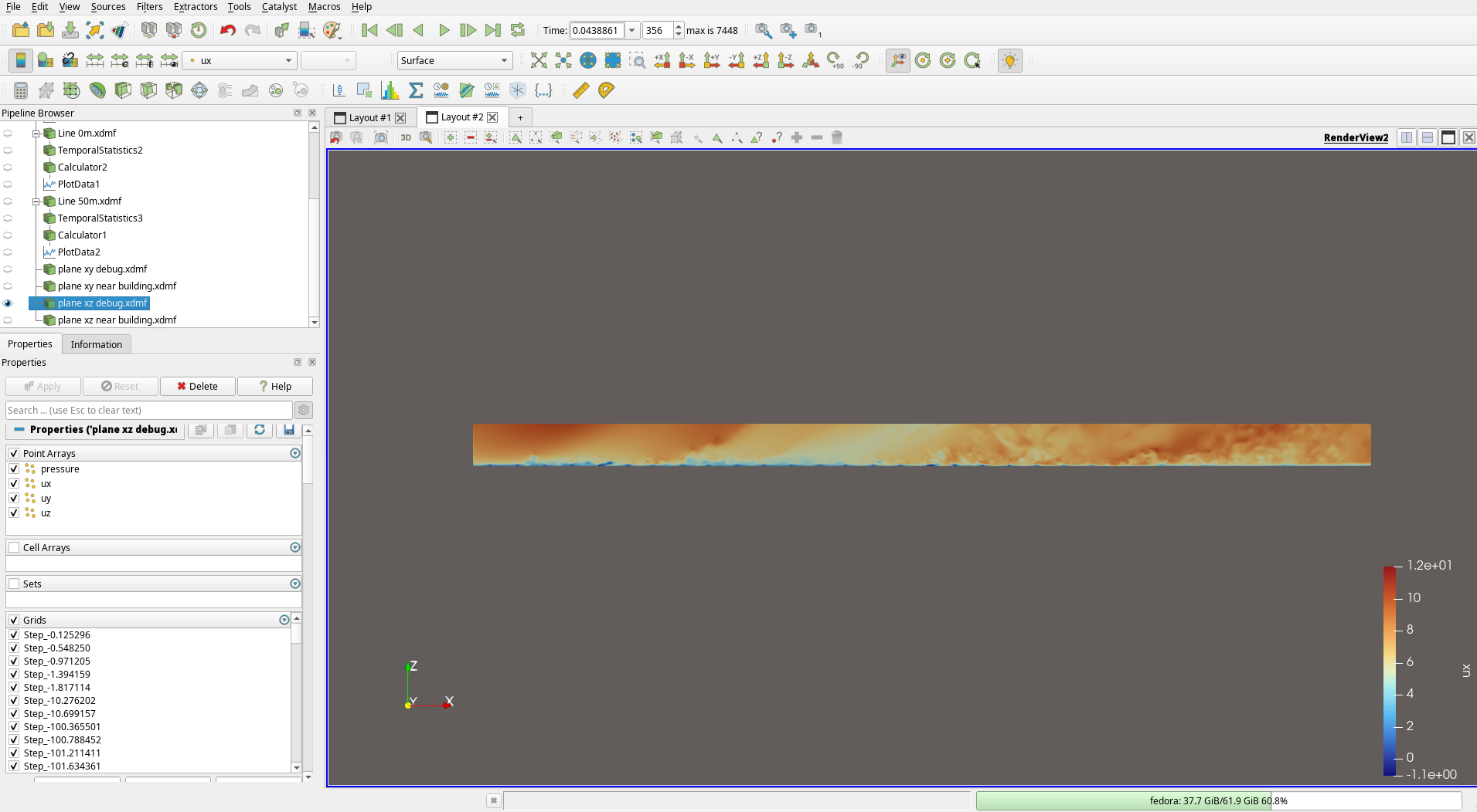
The XZ debug plane coloured by \(u_x\).

We can see that the field seems to be developed.

It’s also interesting to create animations from these, so that we can see the flow evolving overall. By setting the camera, changing colormaps and configuring the lighting, it’s possible to create great animations.

Streamwise velocity on the XZ plane, animated over the acquisition window.

A similar process can be done for the other exports, such as the volume debug, the statistics export, and the other plane exports.

Now we have a basic ABL case, from end to end.