5. Data Exports

We need to set the simulation exports in order to be able to run it. We need exports for viewing the simulation fields, being able to process the results, and also debugging the simulation.

Debug Exports

We highly recommend setting up debug exports for all simulations. A plane debug and a full domain are must-haves, to be able to debug what happened.

To generate full domain exports we go to Exports -> Macroscopics and then add a new one. In the form, we set its name as full domain debug, its type to Volume and activate Full domain. For the export period, we set a high value so as not to generate too much data, 150 s in this case, and select all fields.

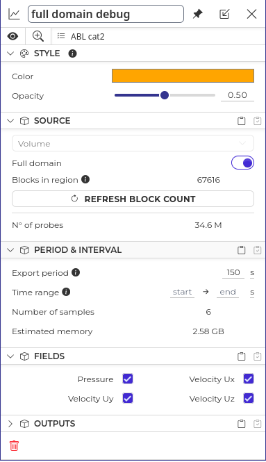
Full domain debug export: all fields, one snapshot every \(150\,\text{s}\).

We recommend generating export planes as well, in the region of interest. For this case, we will add a plane in XY and one in XZ near 0 m, to check the flow and its evolution with a bigger frequency.

First adding the XZ plane, we go to the same path, but now choose Plane instead of Volume. Set the plane normal axis to Y, the axis position to 0 m, the point spacing to 2 m, activate Limit in-plane region and set it from -750 m, 0 m to 300 m, 100 m.

For the export period, we use a period that lets us see the evolution but at the same time does not overgenerate data. For this case we will use 0.5 s, for the time the whole simulation, and for the fields we can select all.

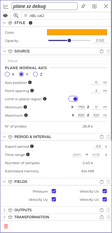
XZ debug plane: normal in Y at \(y = 0\), spanning the region of interest.

Now for the XY plane, we duplicate the XZ plane and just change the normal axis to Z, the axis position to 3 m, and the plane region in Y to -100 m to 100 m.

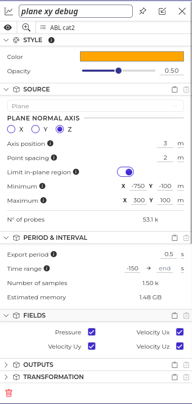
XY debug plane: normal in Z at \(z = 3\,\text{m}\), the reference height.

With this we should have our debug exports set up and can proceed to the ones for processing.

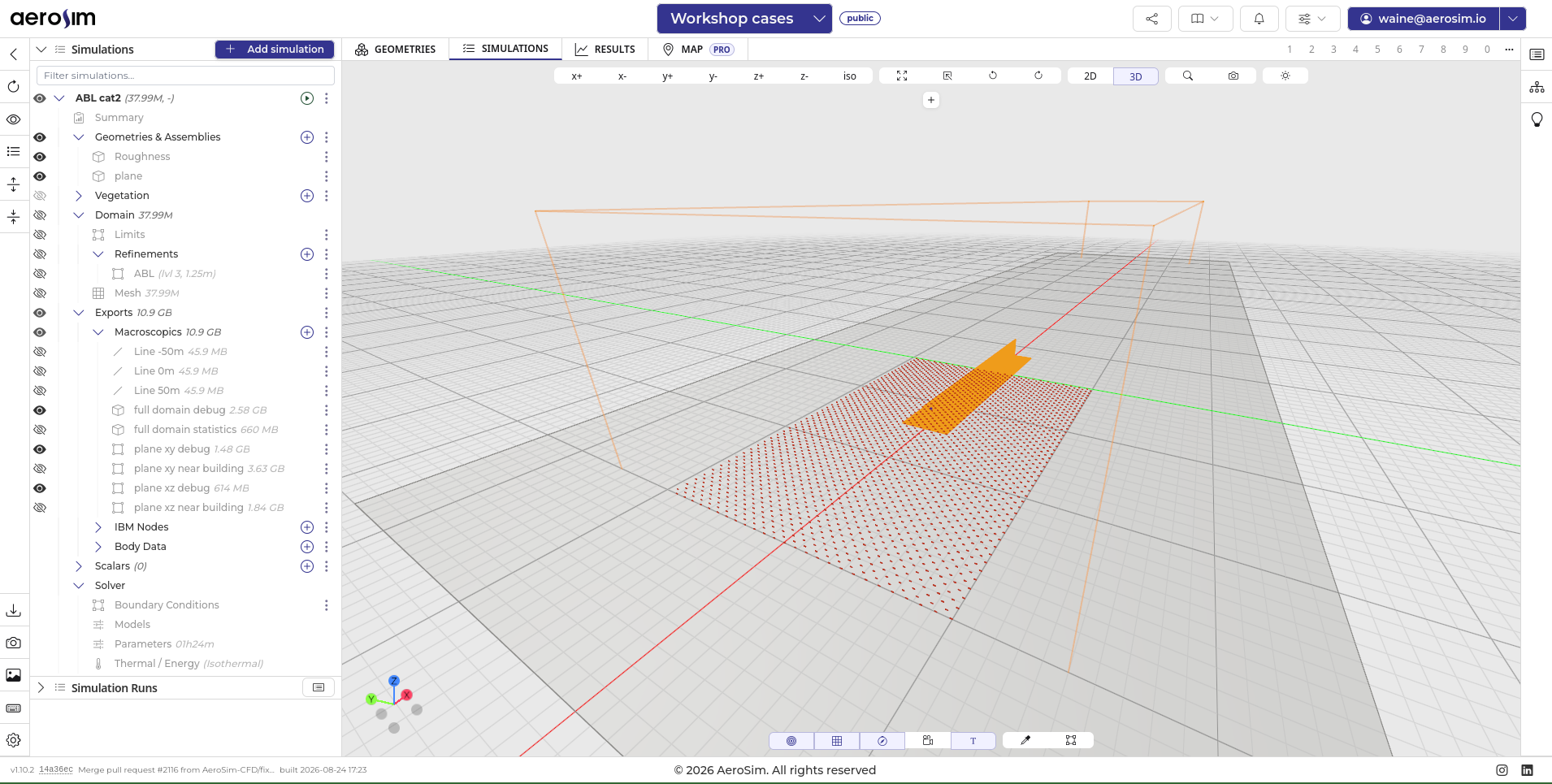
The three debug exports in the simulation tree.

Domain Statistics

For the ABL it is very common to be interested in the average values of the fields. For this, AeroSim exports statistics as well.

In this case we will duplicate the full domain debug, change its name to full domain statistics, set the export period to 1 s and the time range to start at 0 s.

We also need to open Outputs, deselect instantaneous and select statistics, otherwise it will export the whole domain with that period, which would generate tens of GB of data.

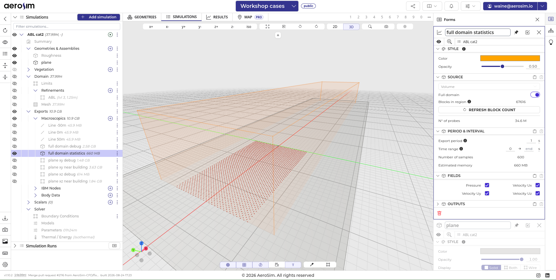
Full domain statistics export, sampling from \(t = 0\,\text{s}\) to the end.

Line Profile

For processing length scales and other transient statistics, it is interesting to have time series of the velocity fields, especially where the bodies are placed.

In this case, we will add lines of exports at 0 m, 50 m and -50 m, to check how the flow is at the centre, downstream and upstream.

For it we will add a line at 0 m, set its start at (0 m, 0 m, 0 m) and end at (0 m, 0 m, 100 m) with 101 points in it. For the export time, set the export period to 0.1 s and the time range to start at 0 s. We can export only velocity or all fields; in this case we chose to export all fields.

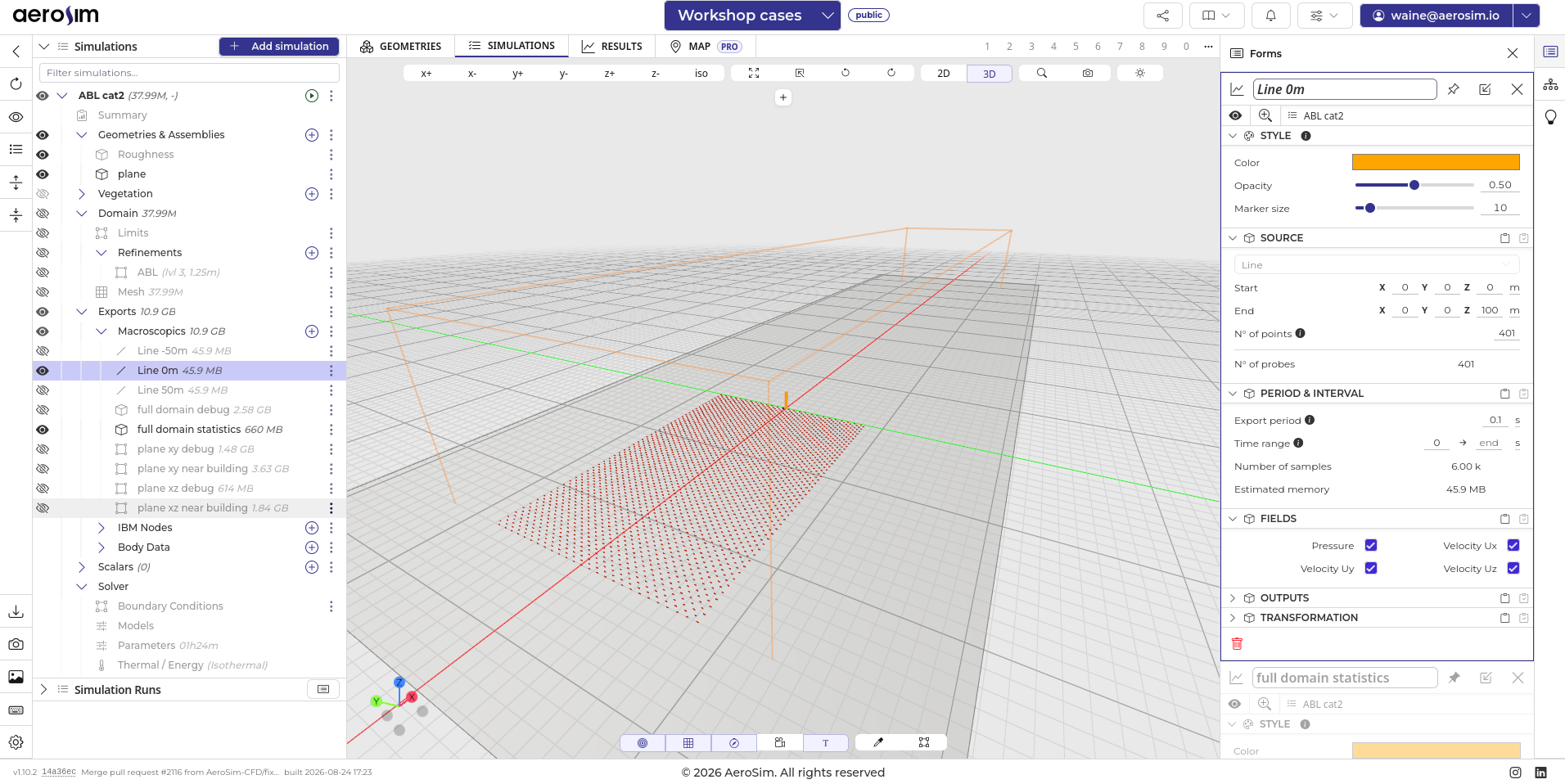
The vertical line export at \(x = 0\), sampled every \(0.1\,\text{s}\).

After that we will duplicate the line and just change the position and the names to -50 m and 50 m. With that, all lines for export are configured.

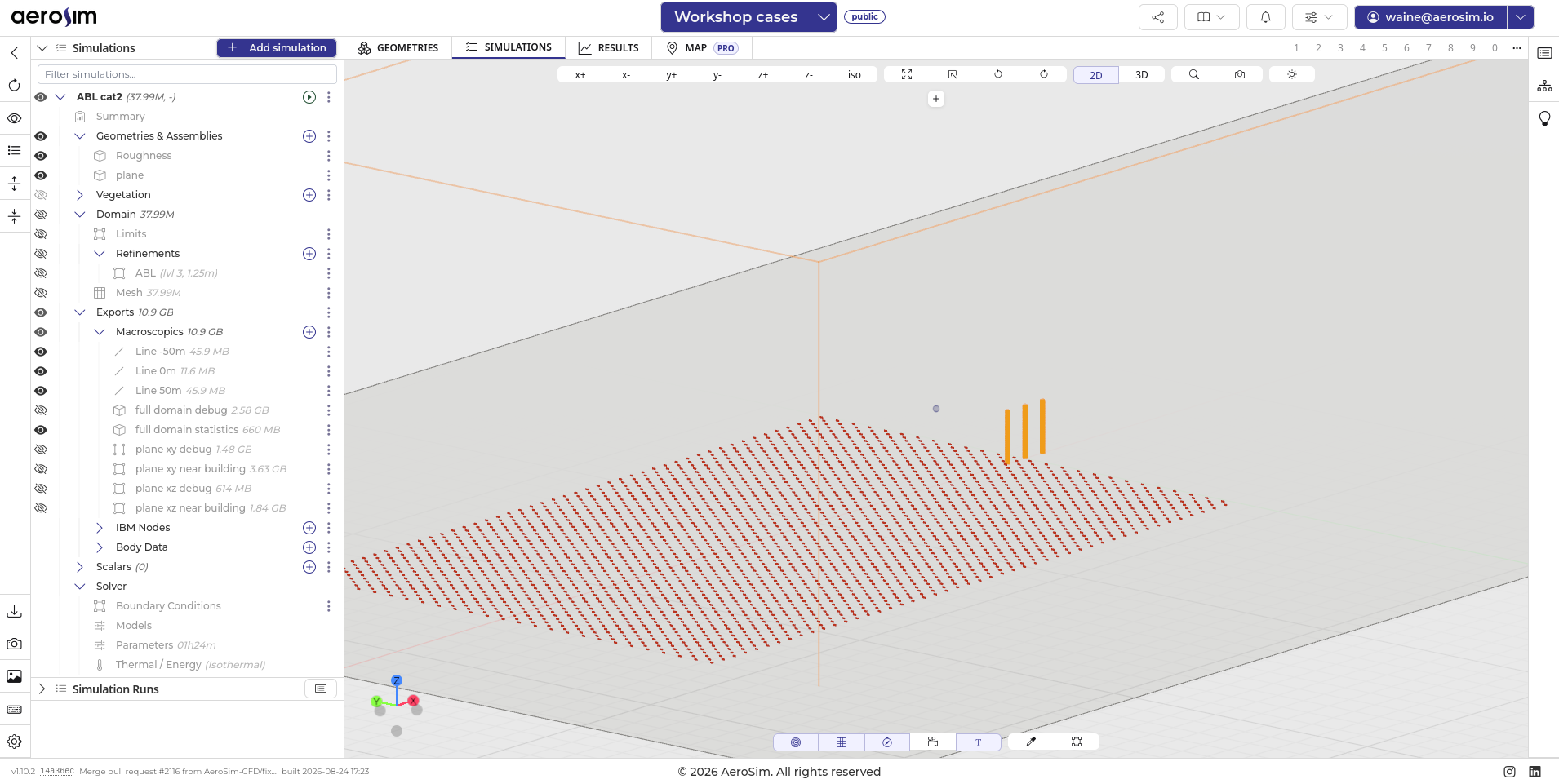
The three vertical lines, at \(x = -50\,\text{m}\), \(0\) and \(50\,\text{m}\).

Other Exports

The above ones are the most common for ABL simulations, but feel free to add other ones that you may be interested in, such as YZ planes, more volumes, streamwise lines, etc.

In this case, to check the flow near the building, we duplicated the debug planes, changed their limits to be near the origin only, changed the resolution, and added a higher sampling to sample only after the simulation development.

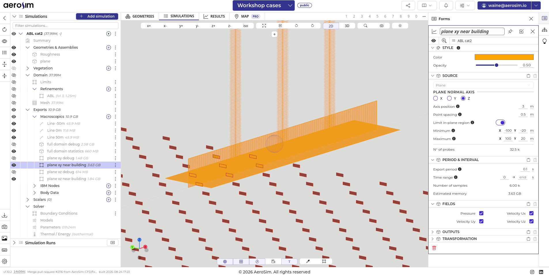
A near-building plane: finer point spacing, tighter limits and a higher sampling rate, starting only at \(t = 0\,\text{s}\).

Next Steps

Now the whole simulation is set up, it’s time to run it.