Immersed boundary method¶

The immersed boundary method (IBM) enables flow simulations over complex obstacles using stationary computational meshes that encompass the solid bodies. The flexibility comes at the price of imposing interpolated boundary conditions on locations in-between the fluid grid nodes.

Why an immersed boundary method¶

A simulation usually starts from a geometry delivered as an arbitrary triangulated surface (an STL file). The flow solver, however, works on the regular Cartesian lattice that the lattice Boltzmann method (LBM) requires, where every node sits on a uniform grid and the streaming step simply shifts populations between neighbours. The central difficulty is reconciling these two worlds: a geometry of arbitrary shape and orientation must impose a no-slip wall condition on a grid whose nodes almost never land on the surface.

The classical answer is a body-fitted mesh: deform and refine the grid so that cells conform to the walls. For a single clean shape this works, but for complex or multi-body geometries it scales badly. Many bodies, sharp corners, and overhangs mean every geometry change forces a full remesh, and the resulting non-uniform, skewed cells are exactly what the LBM streaming step cannot accommodate. The mesh generation effort, not the flow solve, becomes the bottleneck.

The immersed boundary method removes the remeshing step entirely. The body is left immersed in a fixed Cartesian lattice, and its presence is communicated to the fluid through a localized forcing function rather than through the grid topology Mittal and Iaccarino[1]. Because the lattice never changes, the same uniform grid and the same streaming kernel serve any geometry, and swapping one body for another costs nothing on the fluid side. This is what makes IBM a natural fit for the LBM workflow in Nassu: the geometry is decoupled from the solver grid.

Key idea

IBM does not carve the body out of the grid. It leaves the lattice untouched and adds a local force that pushes the fluid to a halt at the wall, so a single uniform-grid kernel enforces no-slip on any geometry.

Note

IBM goes under other names, such as Cartesian grid method, the immersed interface method, the embedded boundary method, the fictitious domain method, etc.

Diffuse versus sharp interface¶

IBM variants differ in how strictly they resolve the wall. Sharp-interface methods reconstruct the geometry to within a grid cell, modifying the discrete operators of the cut cells so the boundary is felt as a crisp line. They are accurate but reintroduce geometry-dependent, case-by-case stencil bookkeeping, which works against the uniform-kernel philosophy of LBM.

Nassu instead uses a diffuse-interface formulation in the lineage of Peskin[2]. The wall is not represented as a discontinuity; the forcing is smeared over a thin band of fluid nodes straddling the surface, a few cells thick. The pay-off is robustness and a single, geometry-independent kernel: every Lagrangian point of every body is handled by the same smoothing operation. The cost is a slightly blurred wall, so very near-wall gradients are resolved over the width of the band rather than over a single cell. For external bluff-body aerodynamics, where the quantities of interest are pressures, separation, and wakes rather than sub-cell wall detail, this trade is favourable, and the residual near-wall error can be further reduced with a wall model (see Combine and Spread).

An optional near-wall viscous correction of Du et al.[3] is also available. It is opt-in and off by default, enabled per IBM body with visc_correction: true in the config, and is only available together with LES (the configuration raises an error if it is requested without an LES model). It is intended to be combined with a wall model and is experimental, so it may cause instabilities; no curated validation case relies on it. It is not applied automatically at near-wall nodes - it must be explicitly enabled.

Diffuse interface vs sharp interface

A sharp-interface method resolves the wall to within a cell but reintroduces per-geometry stencil bookkeeping in the cut cells. The diffuse interface trades that crisp wall for one robust, geometry-independent kernel and a band a few cells thick. Reach for the wall model when the blurred band would otherwise lose the near-wall gradient you need.

Basic Principles¶

An IBM Lagrangian mesh is superposed on an LBM Eulerian grid. The computational points from the Lagrangian mesh are referred to as “solid” nodes. In turn, the “fluid” nodes are those on the Eulerian grid.

To assure a no-slip boundary condition, the IBM uses an extra forcing function that’s distributed over a thin band of neighbouring fluid nodes to take effect (diffuse interface), as illustrated below:

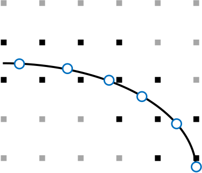
where the black grid nodes represent the thin band over which a correction force \(f_{\alpha}\) calculated on the Lagrangian mesh (blue nodes) is distributed. The force field accounts for the presence of an immersed solid body.

The formulation of the correction force requires an interpolated fluid velocity over the solid node. This information is usually obtained via a combine operation from fluid nodes near the local solid node. While the correction force has to be spread to the near fluid nodes after it has been calculated.

Note

The combine operation is commonly referred as interpolation. However, since many interpolative processes were adopted during the whole algorithm development, we opted to use the combine nomenclature for IBM.

The figure below illustrates the combine and spread operations. The interpolations are obtained by a smoothed delta function.

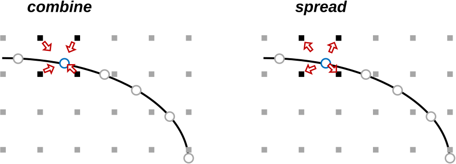
Note

The diffuse interface is defined by the fluid nodes that are affected by the spread operation.

Where IBM sits in the time step¶

The placement of the IBM operations within the LBM cycle is deliberate. After streaming, the solver computes the macroscopic fields (density and velocity) at every fluid node. Only at this point is the velocity near the wall known, so the combine operation reads a meaningful interpolated velocity, the forcing is computed to cancel the slip it finds, and the resulting force is spread back onto the fluid before the collision step folds it into the populations. Running IBM after the macroscopics and before collision is therefore what lets a single time step both measure the wall slip and correct it.

Important

IBM enters the cycle after the macroscopics are computed and before LBM collision. Run it earlier and the combine reads a velocity that does not exist yet; run it later and the spread force never reaches the collision that should feel it.