Smagorinsky

The previous page reduced subgrid modelling to one missing ingredient: a computable estimate of the subgrid velocity scale \(V\). The Smagorinsky model, the oldest and still the most widely used subgrid closure [1], makes the simplest possible choice for it. It is the default subgrid model in Nassu, and this page explains where its formula comes from, what its one constant means, where it is known to fail, and the specific advantage it gains inside the lattice Boltzmann method.

The model

Smagorinsky’s idea is to tie the subgrid velocity scale to the resolved strain rate. If the resolved flow is being sheared strongly, the eddies it spins off, including the unresolved ones, are correspondingly energetic. The natural local measure of that shearing is the magnitude of the resolved rate-of-strain tensor, \(|S| = (2 S_{\alpha\beta} S_{\alpha\beta})^{1/2}\). Combined with the only available length, the filter width \(\Delta x\), this gives a subgrid velocity scale \(V \sim \Delta x\, |S|\), so the subgrid kinetic energy \(k_{\ell}\) is taken to be of order \((\ell |S|)^{2}\). Inserting \(V\) into the dimensional estimate \(\nu_{\mathrm{SGS}} \sim \ell V\) yields

(1)\[\begin{split} \begin{aligned} \nu_{\mathrm{SGS}}&=C_{\mathrm{S}}^{2}\left(\Delta x_{n}\right)^{2}\left(2S_{\alpha\beta}S_{\alpha\beta}\right)^{1/2}\\ S_{\alpha\beta}S_{\alpha\beta}&=S_{xx}^{2}+S_{yy}^{2}+S_{zz}^{2}+2\left(S_{xy}^{2}+S_{xz}^{2}+S_{yz}^{2}\right) \end{aligned} \end{split}\]

The model is purely local and algebraic: everything on the right-hand side is known at the current node and time step from the resolved field, so \(\nu_{\mathrm{SGS}}\) costs almost nothing to evaluate. This cheapness and robustness are why Smagorinsky remains the workhorse closure for engineering LES. Here \(\Delta x_{n}\) is the lattice spacing at refinement level \(n\), which sets the filter width on that block. The bar over the resolved rate-of-strain has been dropped for brevity; \(S_{\alpha\beta}\) here is the resolved strain rate.

The Smagorinsky constant

The single free parameter \(C_{\mathrm{S}}\) sets how much subgrid viscosity the model produces. Its value is not arbitrary: assuming the cut-off lies in the inertial subrange and requiring the model to dissipate energy at exactly the cascade rate of Equation (2), Lilly derived \(C_{\mathrm{S}} \approx 0.17\) for isotropic turbulence [2][3]. This is the value used by default. In practice \(C_{\mathrm{S}}\) is often lowered toward \(0.1\) in sheared and wall-bounded flows, because in those flows the mean shear contributes to \(|S|\) and the standard model becomes over-dissipative, damping the very resolved fluctuations LES is meant to capture [4]. The right value is therefore part of the validation exercise for a given class of flow, not a universal constant.

Choosing the constant

Use \(C_{\mathrm{S}} \approx 0.17\) for free shear and isotropic turbulence, where Lilly’s derivation holds. Lower it toward \(0.1\) for wall-bounded and strongly sheared flows, where the mean shear inflates \(|S|\) and the model otherwise over-dissipates. For a new class of flow, treat \(C_{\mathrm{S}}\) as a parameter to validate, not a constant to assume.

The near-wall deficiency

The Smagorinsky model has a well-known and physically important flaw: it does not switch itself off at a solid wall. As a wall is approached, turbulent fluctuations and hence the true subgrid stress must vanish, because the no-slip condition suppresses the eddies. The model in Equation (1), however, keeps producing \(\nu_{\mathrm{SGS}}\) wherever there is mean shear, and the mean shear is in fact largest at the wall. The result is a spurious subgrid viscosity in the near-wall region that thickens the boundary layer and corrupts the wall shear stress, and with it the surface pressures and friction that set the loads on the body [3][4].

The classical solution is a damping function that forces \(\nu_{\mathrm{SGS}}\) to zero at the wall, the most common being the Van Driest damping originally devised for the mixing length [5]. It multiplies \(C_{\mathrm{S}}\) by a factor that decays with wall distance measured in viscous units, restoring the correct near-wall behaviour. The cost is that it requires the wall distance and the local friction velocity at every node, which is awkward in a method built on a Cartesian lattice with immersed bodies; for that reason near-wall accuracy in Nassu is handled primarily through wall-model boundary conditions rather than a global damping function.

Why not dynamic Smagorinsky

A more elaborate fix is the dynamic Smagorinsky procedure, which computes \(C_{\mathrm{S}}\) locally from the resolved field and so automatically reduces it near walls. It is not used here because it requires an explicit test-filter operation over the resolved variables, which is non-local and expensive on the block-structured grid.

The lattice Boltzmann payoff

So far the model has been described in Navier-Stokes terms, where computing \(\nu_{\mathrm{SGS}}\) requires the strain-rate tensor \(S_{\alpha\beta}\), which in a conventional solver must be reconstructed from velocity gradients by finite differences. The lattice Boltzmann method has a decisive advantage here. The strain rate is already available locally, encoded in the non-equilibrium part of the populations, with no spatial gradients to compute [6]. Concretely, the strain rate can be written as

(2)\[ S_{\alpha\beta}=-\frac{\omega}{2\rho c_{s}^{2}\Delta t}Q_{\alpha\beta} \]

where the tensor \(Q_{\alpha\beta}\) collects the non-equilibrium stress and the force contribution,

(3)\[ Q_{\alpha\beta}=\Pi_{\alpha\beta}^{\mathrm{neq}}+\frac{\Delta t}{2}\left(F_{\alpha}u_{\beta}+F_{\beta}u_{\alpha}\right) \]

and both \(\Pi_{\alpha\beta}^{\mathrm{neq}}\) and the force term are known at the node from the collision step.

This locality unlocks a second, more important simplification. In an LES the effective relaxation time is \(\tau^{*}=\tau + \Delta\tau\), and the increment \(\Delta\tau\) depends on \(\nu_{\mathrm{SGS}}\), which through Equation (1) depends on \(|S|\), which through Equation (2) depends on \(\tau^{*}\) again. The relaxation time appears on both sides, so in a conventional formulation it would have to be found by iteration at every node and every step. Because the dependence is only quadratic, Dong et al.[6] showed it can instead be solved in closed form, giving an explicit expression for the effective relaxation time:

(4)\[ \tau^{*}=\frac{1}{2}\left(\tau+\sqrt{\tau^{2}+\frac{2C_{\mathrm{S}}^{2}\left(\Delta x_{n}\right)^{2}\sqrt{2Q_{\alpha\beta}Q_{\alpha\beta}}}{\Delta t \rho c_{s}^{4}}}\right) \]

This is what Nassu actually computes. At each node and step the solver forms \(Q_{\alpha\beta}\) from the local non-equilibrium stress, evaluates the square root in Equation (4) directly, and uses the resulting \(\tau^{*}\) to recover the filtered macroscopic variables and to carry out the collision. No velocity gradients, no neighbour communication for the strain rate, and no inner iteration are required, which is precisely what makes Smagorinsky LES cheap enough to run at high Reynolds number and over large domains.

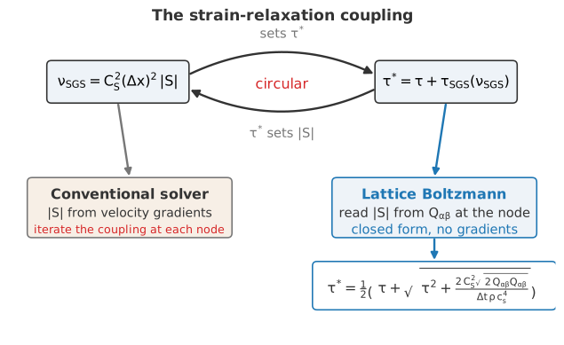
The strain-to-viscosity closure on the lattice. The subgrid viscosity depends on the strain-rate magnitude \(|S|\), which couples back into the relaxation time. A conventional solver must iterate this coupling; the lattice Boltzmann method instead reads \(|S|\) directly from the non-equilibrium stress \(Q_{\alpha\beta}\) at each node, with no velocity gradients, giving a closed-form relaxation time.

Why a regularized operator and not plain BGK

The strain rate the model reads comes straight from the non-equilibrium stress \(Q_{\alpha\beta}\), so that stress must stay clean. The plain BGK operator pollutes it with spurious high-order moments, corrupting the very \(|S|\) fed to Equation (1) and making Equation (4) untrustworthy [7]. Reconstructing the populations on a Hermite basis before collision removes this contamination, which is why a regularized operator is essential, not optional, for reliable LBM-LES.

---

[1]

Joseph Smagorinsky. General circulation experiments with the primitive equations: I. The basic experiment. Monthly Weather Review, 91(3):99–164, 1963. doi:10.1175/1520-0493(1963)091<0099:GCEWTP>2.3.CO;2.

[2]

Douglas K. Lilly. The representation of small-scale turbulence in numerical simulation experiments. Proceedings of the IBM Scientific Computing Symposium on Environmental Sciences, pages 195–210, 1967.

[3] (1,2)

Stephen B. Pope. Turbulent Flows. Cambridge University Press, 2000. doi:10.1017/CBO9780511840531.

[4] (1,2)

Pierre Sagaut. Large Eddy Simulation for Incompressible Flows: An Introduction. Scientific Computation. Springer-Verlag, Berlin Heidelberg, 3 edition, 2006. doi:10.1007/b137536.

[5]

Edward R Van Driest. On turbulent flow near a wall. Journal of the aeronautical sciences, 23(11):1007–1011, 1956.

[6] (1,2)

Yu-Hong Dong, Pierre Sagaut, and Simon Marie. Inertial consistent subgrid model for large-eddy simulation based on the lattice Boltzmann method. Physics of Fluids, 20(3):035104, 2008. doi:10.1063/1.2842379.

[7]

Patrick Nathen, Daniel Gaudlitz, Mathias J. Krause, and Nikolaus A. Adams. On the stability and accuracy of the BGK, MRT and RLB Boltzmann schemes for the simulation of turbulent flows. Communications in Computational Physics, 23(3):846–876, 2018. doi:10.4208/cicp.OA-2016-0229.