
 AeroSim Docs
Multiblock
The multiblock feature allows for subdivision of the computational domain in finer grid refinement regions. This is illustrated by the figure below
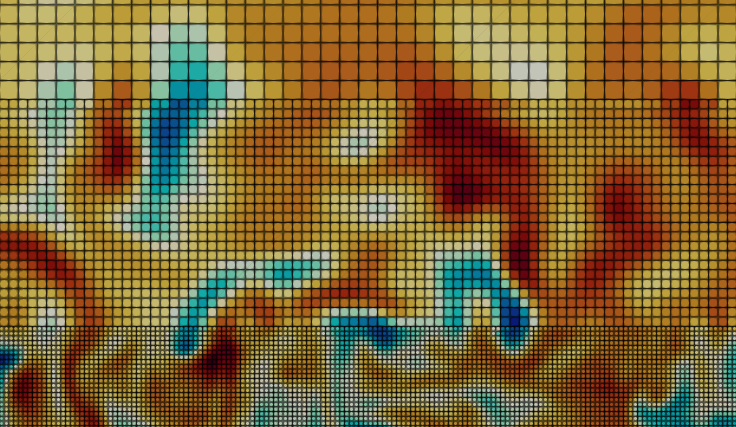
Multiblock example
The refinement structure is separated in levels whose resolution is always double the previous level, beginning at level 0.
The transition between levels must always occur from a previous to a next level (e.g: a transition from level 1 to level 3 must include a level 2 region in-between).
The refined regions are determined in domain.refinement field:
    domain:
      refinement:
        static:
          volume_refinement_lvl1:
            volumes_refine:
              - is_abs: true
                lvl: 1
                start: [0.0, 0.0, 0.0]
                end: [32.0, 160.0, 64.0]
            volumes_not_refine:
              - is_abs: false
                start: [0, 0.15, 0.1]
                end: [0.1, 0.2, 0.3]
          body_refinement_lvl3:
            bodies:
              - body_name: solid-body1
                lvl: 3
                normal_offsets: !range [-0.25, 0.2501, 0.125]
            volume_refinement_limit:
              is_abs: true
              start: [0, 10, 0]
              end: [40, 50, 150]
Important
It is recommended to avoid placing too many Lagrangian mesh nodes in the level transition regions. Hence when using the body refinement, an offset interval of at least +/- 1 block may be necessary.
To fill the regions between offset limits, we suggest to use !range as shown above.
Corners are read in the frame the entry declares. With is_abs: true they are absolute lattice coordinates (optionally written in a domain.systems frame through system); with is_abs: false they are fractions of the domain, so 0.25 is a quarter of the way across. A volume whose resolved box misses the domain, or is thinner than one level-0 node on any axis, is rejected at setup - a box that thin selects blocks by a sliver and is almost always relative corners left tagged as absolute.
Graduated transition margins
A refinement region drops to level 0 immediately outside its box, which puts the coarsest grid right next to the finest. lattice_margin softens that by adding one transition shell per intermediate level: the shell at each level below the target reaches a given number of nodes of that level’s own spacing further out than the previous one. A margin of m on a level-3 volume therefore extends the level-2 shell by m/4 and the level-1 shell by a further m/2 in level-0 units.
A volume names its margin per face; a body names it along the surface normal, with outer growing away from the body and inner into it. The two mean the same distance: a body margin of m and a volume margin of m grow the refined region by the same amount.
    domain:
      refinement:
        static:
          graduated:
            volumes_refine:
              - is_abs: true
                lvl: 3
                start: [96, 96, 96]
                end: [160, 160, 160]
                lattice_margin:
                  x_neg: 32
                  x_pos: 32
                  y_neg: 24
                  y_pos: 24
                  z_neg: 0
                  z_pos: 16
                  margin_stop_lvl: 0
            bodies:
              - body_name: solid-body1
                lvl: 3
                normal_offsets: [0]
                lattice_margin:
                  inner: 0 # do not refine into the solid
                  outer: 32
                  margin_stop_lvl: 0
margin_stop_lvl stops the graduation: levels at or below it get no shell. The default 0 adds shells all the way down to level 1.
Important
Refinement selects whole blocks, and the 2:1 grading rule already puts about two blocks of transition around a refined region. A margin has to exceed roughly 2 * block_size nodes at a level’s own spacing before it widens anything. Setup logs the shell widths it requested and how many blocks they added, and warns when a margin added none - if that warning appears, raise the margin or drop it.
Leaving inner at 0 matters for a closed body: the outer margin still grows the shell tangentially along the surface, but nothing is refined deeper into a solid interior, whose nodes do not take part in the solution.
Oriented (rotated) refinement volumes
By default a refinement volume is axis-aligned: its start/end corners are read directly in domain coordinates. To refine a region that sits at an angle to the domain axes (for example a tight box hugging a rotated building), add an optional transformation. The start/end corners then define the box in a local frame and the transformation maps it into the domain, producing an oriented box.
    domain:
      refinement:
        static:
          oriented_volume:
            volumes_refine:
              - is_abs: true # required when a rotation is given
                lvl: 4
                start: [0, 0, 0]
                end: [40, 20, 60]
                transformation:
                  rotation: [0.0, 0.0, 0.7853981634] # 45 deg about z (radians)
                  translation: [60.0, 40.0, 0.0]
                  fixed_point: [20.0, 10.0, 30.0] # box centre
The transformation fields (rotation in radians, translation, fixed_point, scale) match the body transformation, so a refinement volume and a body can share the same transformation and stay co-located. When transformation is omitted the volume stays axis-aligned. The same transformation field is also accepted on export, monitor and statistics volumes.
Note
A non-zero rotation requires is_abs: true: a rotated box can only be interpreted unambiguously in absolute coordinates. lattice_margin shells expand the box in its local frame and are mapped through the same transformation.
On an export volume the transformation does two things: it selects the blocks overlapping the oriented box (as for refinement), and it rigidly transforms the exported geometry so the volume is written rotated in space. The transform is applied to the output node coordinates on top of the global export rescale, and the affected blocks are emitted as an explicit structured grid (XDMF 3DSMesh, a vtkStructuredGrid) so the orientation survives into ParaView. The macroscopic values are written unchanged - there is no resampling onto a new grid, only the coordinates move. An export volume with no transformation keeps the regular axis-aligned grid (3DCoRectMesh) and its output is unchanged.
Overlap F2C
In the current multiblock framework, the communication between coarse and fine level requires an overlap of both grids, as shown below:
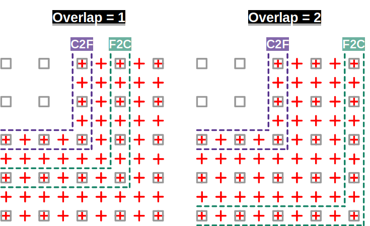
Overlap in F2C (fine to coarse)
Important
For turbulent flows, it is common practice to use at least 2 nodes for the overlap to provide certain flow development between level transitions.
This configuration is set in the models.multiblock field:
      multiblock:
        overlap_F2C: 2
        # It's possible to define custom overlaps of F2C for specific levels
        # To do so, use as [lvl_from]: overlap to use
        custom_overlap_F2C:
          1: 3
          2: 3
          5: 1
Interface coupling scheme
The operator that couples coarse and fine grids at a refinement interface is selected with models.multiblock.interface_coupling:
      multiblock:
        interface_coupling: value_interp   # or: conservative
value_interp(default) is the value-interpolation coupling: a cubic four-point coarse-to-fine prolongation of the macroscopics and a fine-to-coarse point injection.conservativereplaces the transfer of the fluid conserved moments (density and momentum) with a conservative pair on the same 2:1 nodes: a positivity-preserving momentum-space prolongation (density and momentum are interpolated with convex weights and the velocity is recovered as momentum over density) and a fine-to-coarse restriction that averages the fine children. The non-equilibrium stress channel, its LES stress rescaling and the temporal interpolation are shared by both schemes.
The conservative scheme keeps mass and momentum continuous across the interface, which forbids the negative-density interface failure that the cubic prolongation can produce in strong turbulence at near-inviscid relaxation. On smooth flows it recovers the interface momentum the value interpolation loses: for a laminar channel with a refinement interface across the flow, the peak-velocity error against the analytical parabola drops from about 4% to below 1%. The operator definitions are given in the multiblock communication theory page.
Note
interface_coupling: conservative currently applies the conservative transfer to the fluid density and momentum. Transported scalar and energy fields keep their existing interface transfer under either setting.
Interface checkerboard stabilization
At near-inviscid relaxation (omega -> 2) in strong turbulence, a refinement interface can excite a grid-scale (2dx) odd-even checkerboard mode that grows and diverges. The optional models.multiblock.interface_stabilization adds an adaptive dissipation that suppresses this mode without over-dissipating the resolved flow:
      multiblock:
        interface_coupling: conservative
        interface_stabilization:
          strength: 0.2    # extra-viscosity gain (a local Smagorinsky-constant boost)
          threshold: 0.5   # sensor value (0 smooth, 1 grid-scale) above which it ramps in
A per-node 2dx odd-even (Jameson) sensor measures how much of the local field is the grid-scale mode (0 for smooth flow, approaching 1 for a pure checkerboard). Where the sensor exceeds threshold, a graded extra subgrid viscosity strength^2 * |S| * gate is added through the LES relaxation - a local boost of the Smagorinsky constant. Because the sensor distinguishes the checkerboard from physical shear, the extra dissipation is inactive in smooth resolved flow (a smooth laminar profile is unchanged to within rounding), so it localizes the global-Cs cure to where it is needed. It requires models.LES; omitting it disables the feature and leaves the generated kernels byte-identical.
Important
strength has a working window: too small does not suppress the mode, too large introduces its own near-interface viscosity discontinuity that can diverge sooner. A value comparable to the base Smagorinsky constant is a good starting point; pair it with interface_coupling: conservative, which already reduces the dissipation needed.
Saving and loading a BlockForest
Building the BlockForest from the YAML refinement program is the dominant cost
at simulation startup for non-trivial CWE cases. To avoid replaying the
divide_volume / divide_geometry calls every time, the forest can be
serialised to disk and reloaded:
from nassu.api import load_block_forest
from nassu.LBM import VelocitySet
from nassu.multiblock import BlockForest

vel_set = VelocitySet("D3Q27")
bf = BlockForest(vel_set, (256, 128, 128), 8, (False, False, False))
# ... apply divide_volume / divide_geometry as usual ...

bf.save("mygrid.nassu-bf")          # writes mygrid.nassu-bf.json
bf2 = load_block_forest("mygrid.nassu-bf.json", vel_set)
The output is a single self-describing JSON file with a .nassu-bf.json
extension. The domain header (dimensionality, periodicity, refinement levels,
block counts, etc.) is human-readable; the per-block records are stored as a
base64-encoded binary payload at the end of the object so a head or jq
inspection workflow shows the readable fields first:
jq 'del(.blocks.encoded_payload_b64)' mygrid.nassu-bf.json
Integrity is verified on load via SHA-256 of the decoded payload, and the
loader cross-checks vel_set.dim against the file’s dim field. Loading a
file written by an incompatible Nassu version (different JSON schema or block
record layout version) raises BlockForestFormatError rather than silently
loading garbage.
Note
Only the grid topology is serialised - boundary-condition assignments, populations, macroscopics, and any other simulation state are not part of the file and are rebuilt as usual when the forest is loaded.
From the config file
The save/load primitive is wired into the domain block so the build-once /
reuse loop works entirely from YAML, with no Python glue:
    domain:
      domain_size: {x: 512, y: 256, z: 256}
      block_size: 8
      # Write the constructed forest after the refinement program runs.
      block_forest_save: !sub "${NASSU_FILE_FOLDER}/grids/city.nassu-bf.json"
      refinement:
        static:
          city:
            bodies:
              - {body_name: city, lvl: 3, normal_offsets: [0.0]}
      bodies:
        city: {geometry_path: !sub "${NASSU_FILE_FOLDER}/city.lnas"}
A later run points block_forest_load at the saved file to skip the
re-refinement entirely:
    domain:
      domain_size: {x: 512, y: 256, z: 256}
      block_size: 8
      block_forest_load: !sub "${NASSU_FILE_FOLDER}/grids/city.nassu-bf.json"
The declared
domain_size,block_sizeand periodic dimensions are cross-checked against the loaded file; a mismatch is a configuration error (the loaded forest is authoritative for the base grid).Any
refinement.staticdeclared alongsideblock_forest_loadis applied on top of the loaded forest. This lets you reuse a cached grid and refine it further (for example, add a finer box around a new region of interest) without rebuilding from scratch. For pure reuse, omitrefinemententirely.block_forest_saveandblock_forest_loadare independent; relative paths follow the same convention asgeometry_path(use${NASSU_FILE_FOLDER}to anchor to the config folder).
Estimating disk storage from Python
See also
This section is the narrative how-to. For the full nassu.api surface (every
function, its signature and the result types), see the
Python API reference.
nassu.api.preview_simulation_storage mirrors the nassu preview --storage
CLI flag for notebook and submission tooling that already has a
SimulationConfigs and a BlockForest in hand. The helper is GPU-free and
does not build a SimulationModulesHandler or MacrsHandler: macroscopic
instance counts and the per-element itemsize come directly from
sim_cfg.models. It runs in seconds even on huge cases:
from nassu.api import load_block_forest, preview_simulation_storage
from nassu.cfg.model import ConfigScheme
from nassu.LBM import VelocitySet

sim_cfg = ConfigScheme.sim_cfgs_from_file("my_case.nassu.yaml")[0]
bf = load_block_forest("my_case.nassu-bf.json", VelocitySet("D3Q27"))
estimate = preview_simulation_storage(sim_cfg, bf)
print(estimate.total_bytes, "bytes")
for entry in estimate.by_output:
    print(entry.name, entry.kind, entry.total_bytes)
Pass ibm_node_counts / probe_point_counts to cover bodies and file-backed
probes the helper cannot enumerate from the config alone. Like the CLI, the
estimate ignores compression and per-format overhead - it is the same rough
number you would get from nassu preview --storage.
Per-output composable helpers
For callers that only need to size a single output (a probe series, a
specific instantaneous export, a monitor, etc.) without computing the
whole-sim aggregate, the per-kind helpers are re-exported on nassu.api:
estimate_instantaneous_storage(name, cfg, sim_cfg, block_forest)estimate_stats_storage(name, cfg, sim_cfg, block_forest)estimate_series_storage(name, cfg, sim_cfg)(alias ofestimate_instantaneous_storagefor series targets)estimate_monitor_storage(field_name, cfg, sim_cfg)estimate_ibm_nodes_storage(name, cfg, sim_cfg)
Each takes one data.exports.<name> entry (cfg) and returns a single
OutputStorageEstimate matching the corresponding entry in
preview_simulation_storage(...).by_output (named exports.<name>.{instantaneous,stats}).
All accept an optional macr_itemsize keyword to override the precision derived from sim_cfg,
which is handy for “what-if I switch to single precision” sizing studies without rebuilding the
config:
from nassu.api import estimate_series_storage

series_cfg = sim_cfg.data.exports["line_inlet"]
est = estimate_series_storage("line_inlet", series_cfg, sim_cfg)
print(est.total_bytes, est.n_export_steps, est.n_points)
The pure counters count_volume_nodes, count_points_in_line and
count_series_points, the precision helper macr_itemsize_from_precision
and the macroscopic resolver resolve_macr_instance_names are also exposed
on nassu.api for sizing checks that do not need a byte tally.
Naming convention:
preview_simulation_storage- the whole-sim entry point.estimate_<kind>_storage- per-output composable helpers.count_<thing>- pure counters.resolve_macr_instance_names- the macroscopic resolver.
Estimating GPU memory from Python
See also
The Python API reference is the structured reference for the
whole nassu.api surface, including the memory result types.
nassu.api.preview_simulation_memory is the device-memory counterpart of
preview_simulation_storage, mirroring the GPU-memory figure that nassu preview reports. It is GPU-free and handler-free in exactly the same way -
macroscopic instance counts and the per-element itemsize come straight from
sim_cfg.models, so a notebook or submission UI can size device memory from a
SimulationConfigs plus a BlockForest alone:
from nassu.api import load_block_forest, preview_simulation_memory
from nassu.cfg.model import ConfigScheme
from nassu.LBM import VelocitySet

sim_cfg = ConfigScheme.sim_cfgs_from_file("my_case.nassu.yaml")[0]
bf = load_block_forest("my_case.nassu-bf.json", VelocitySet("D3Q27"))
estimate = preview_simulation_memory(sim_cfg, bf)
print(estimate.total_bytes, "bytes")
for family in estimate.by_family:
    print(family.family, family.n_bytes)
    for component in family.by_item:
        print("  ", component.name, component.n_bytes)
The estimate is broken down per GPU buffer family - macrs (one component per
stored macroscopic group), populations (the border/halo shell), scalar (one
component per models.scalar_transports field), lattice_map, optionally ibm,
and a rough overhead residual given as an explicit, labelled line. Transported
(scalar / DDF) fields are counted by
default. The figure is rough in the same spirit as the CLI: dominant consumers
are explicit, the rest is the overhead residual.
Exact IBM accounting
Pass exact=True together with ibm_node_counts={body_name: n_nodes} to size
the per-body IBM Lagrangian-node device arrays explicitly instead of folding
them into the overhead residual. This mirrors nassu preview --exact-memory
(which collects the node counts off the live setup for you):
estimate = preview_simulation_memory(
    sim_cfg, bf, exact=True, ibm_node_counts={"building": 12000}
)
Per-family composable helpers
For callers that only need to size one family, the per-family helpers are
re-exported on nassu.api, each returning a single MemoryFamilyEstimate:
estimate_macrs_memory(sim_cfg, block_forest)estimate_populations_memory(sim_cfg, block_forest)estimate_scalar_memory(sim_cfg, block_forest)estimate_lattice_map_memory(block_forest)estimate_ibm_memory(sim_cfg, ibm_node_counts=...)estimate_overhead_memory(sized_total_bytes)
All accept an optional macr_itemsize keyword (where applicable) to override
the precision derived from sim_cfg, matching the storage helpers.