Post Processing
After running a simulation, multiple artifacts are generated from it.
These include macroscopics fields exported during simulation, .stl files representing the geometries in the domain, log messages, runtime informations, among many other files.
In this section the output folder structure and files will be explained, as how to interact with them.
Output structure
Each simulation is saved in the folder <save_path>/<simulation_name>/<sim_id>/.
This folder is structured as
📂 save_path/simulation_name/sim_id
  📂 checkpoints
    # Checkpoints saved during simulation, can be used to restart at given step
    📂 {time_step}
      # Macroscopics in the given time step required to restart simulation (rho, u, S, omega_LES)
      📂 macrs
        🗎 {file identifier}.vti
      🗎 macrs.vtm
      # Copy of the simulation's probes folder
      📂 probes
        ...
      # Simulation state required to restart simulation
      🗎 state.json
      # Copy of current log
      🗎 simulation.log
      # Copy of configuration from simulation
      🗎 config.yaml
  📂 bodies
    📂 lnas
      # .lnas is the original file, and transformed
      # is after all transformations applied
      🗎 {body name}.lnas
      🗎 {body name}.transformed.lnas
    📂 nodes
      # Folder for each body, with the IBM nodes positions and their
      # values exports through simulation
      📂 {body_name}
        🗎 nodes.csv
        🗎 {time step export}.csv
    📂 stls
      # STL files for all geometries, after all transformations
      🗎 {body name}.stl
      # STL rescaled to `domain_rescale` scale
      🗎 {body name}.rescaled.stl
  📂 code_generated
    # Each program generated for runtime and its compile log
    🗎 {program name}.cu
    🗎 {program name}.cu.compile.log
  # Macroscopics fields exported
  📂 macrs
    📂 instantaneous
      # Each instantaneous key for export has a folder of its own
      📂 {export name}
        # Each time step export has a .vtm file and a folder
        # with the .vti files used by the .vtm
        📂 macrs_{time_step}
          🗎 {file identifier}.vti
        🗎 macrs_{time step}.vtm
    📂 stats
      # Each statistics key for export has a folder of its own
      📂 {export name}
        # Each time step export has a .vtm file and a folder
        # with the .vti files used by the .vtm
        📂 macrs_{time_step}
          🗎 {file identifier}.vti
        🗎 macrs_{time step}.vtm
  # Monitors exported
  📂 monitors
    📂 fields
      🗎 {monitor name}.{macr_name}.csv
      🗎 {monitor name}.{macr_name}.plot.png
  📂 multiblock
    # File to visualize domain refinement
    🗎 blocks.obj
  # Probes exported
  📂 probes
    📂 hist_series
      📂 {series name}
        # Files for each type, lines, bodies, csvs, points, etc.
        # Each one with .csv for the points of the
        # series and a HDF with time series data for each macroscopics
        # The points position are the ones after all transformations
        🗎 line.{line name}.{macr_name}.h5
        🗎 line.{line name}.points.csv
        🗎 bodies.{body name}.{macr_name}.h5
        🗎 bodies.{body name}.points.csv
        🗎 points.{point name}.{macr_name}.h5
        🗎 points.{point name}.points.csv
        🗎 csvs.{csv name}.{macr_name}.h5
        🗎 csvs.{csv name}.points.csv
    📂 spectrum
      📂 {spectrum name}
        # HDF file with the time series values
        🗎 {spectrum name}.data.h5
        # Point position in the domain
        🗎 {spectrum name}.points.csv
  # Full configuration for simulation
  # (not the same as the original configuration file that generated the simulations)
  🗎 config.yaml
  # Runtime informations for simulation
  🗎 info.yaml
  # Log file
  🗎 simulation.log
Series indexing
There are some specific rules to the historic series indexing that it’s very important to understand to operate with it.
The points are generated using the specification of the generator, then the points outside the domain are filtered out.
The idx field of the points are generated using as reference the initial points (the ones not filtered out).
So, for example, if the first two points of a line are out of the domain, the first index of the points.csv will be 2.
This is important for when you’re combining the idx of this with other sources of information, such as the LNAS vertices or triangles.
Domain overview
To have an overview of the domain setup, we recommend using ParaView. It supports all our file extensions and have extensive funcionalities for visualization, process and many other resources.
Below is an example of domain visualization using the multiblock/blocks.obj and the geometry files of the bodies.
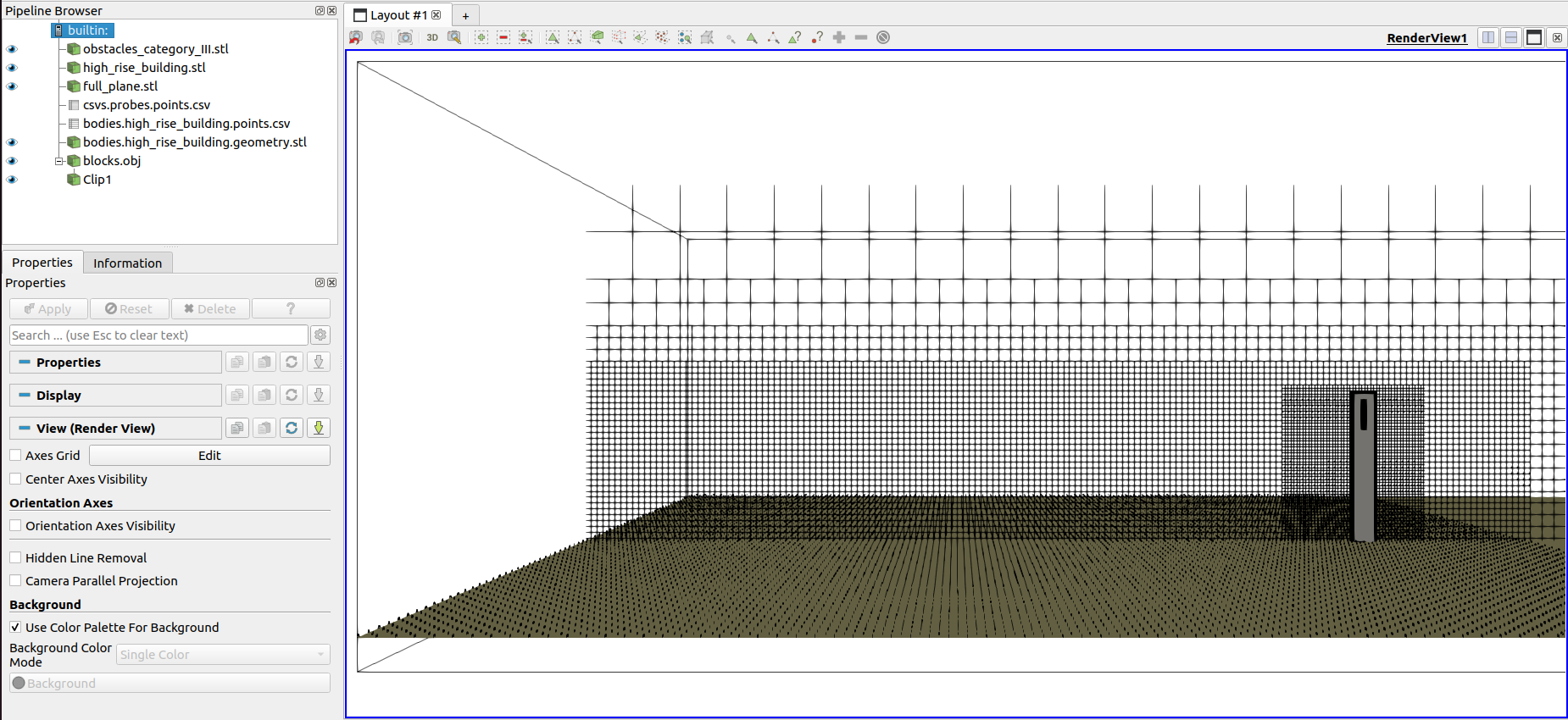
Visualization of domain refinement and positioned bodies
It’s also possible to view the points of series in the domain, converting the csv table to points in space
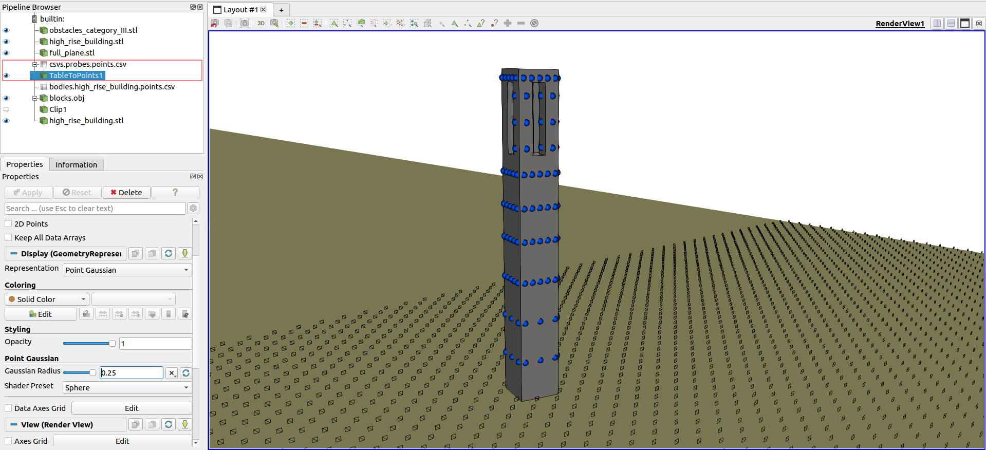
Visualization of points position from historic series
Macroscopics Fields
Check the state of the macroscopics fields, such as density or velocity, is a must step to check the quality of a simulation.
We also recommend ParaView for this.
The macroscopic field can be either exported for instantaneous and statistical values of the macroscopic variables rho, u, S, omega_LES.
The resulting .vtm can be further post processed with Paraview using the calculator tool, as demonstrated below for a statistics field:
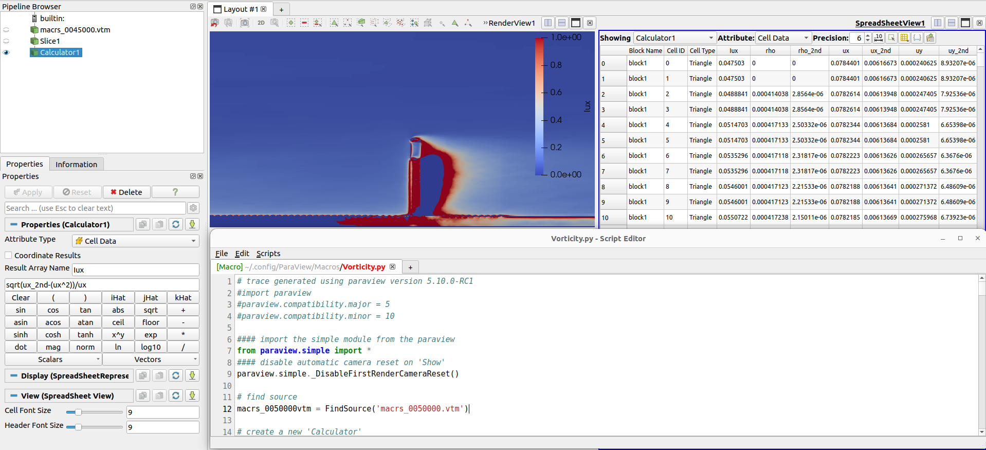
Post processing of macroscopic fields with Paraview
In the example above, the the calculator filter from Paraview is used for the calculation of turbulent intensity \(I_{u}\) from averaged fields of velocity and squared velocity sqrt(ux_2nd-(ux^2))/ux.
Another frequently performed calculation is to transform the velocity components into a vector, which can be done with iHat*ux + jHat*uy + kHat*uz.
Being a Python based software, Paraview allows the user to apply any of its filters through scripts.
This allows the user to write post processing routines that can be performed in any .vtm files that contain the same variable names.
API interaction
All these files and paths can be accessed through an internal API as well. In this way a program can access the full path of files such as the historic series data or points, macroscopics instataneous path, the .obj file with blocks visualization, and other informations.
Below is a code snippet demonstrating how to use it.
import pathlib
from nassu.cfg.model import ConfigScheme
from nassu.cfg.schemes.simul import SimulationConfigs, SimulationOutput

filename = "tests/validation/cases/08_flow_over_mounted_cube.yaml"

sim_cfgs = ConfigScheme.from_file(pathlib.Path(filename)).load_sim_cfgs()
sim_cfg = sim_cfgs[0]
sim_output: SimulationOutput = sim_cfg.output

cube_stl_path = sim_output.bodies["cube"].stl # Path for stl output file of cube
full_info = sim_output.read_info() # reads info.yaml
To know more about this interface and how to interact with it, check the class nassu.cfg.schemes.simul.SimulationOutput.