Meshing

To represent a geometry in the domain, such as a body, Nassu needs to process its geometry into the solver mesh format, a process called meshing. This is done by transforming the body’s representation, given by a .lnas file, into a cloud of points in the domain.

Note

The format for Nassu geometry is a .lnas file, Lagrangian Nassu. It’s the representation of a series of triangles, similar to the .stl format, and support the specifications of surfaces for it.

You can know more about .lnas and how to generate them in stl2lnas repository.

These geometries are defined by the domain.bodies field in the configuration file

simulation:
  - name: BuildingSimulation

    domain:
      bodies:
        solid-body1:
          geometry_path: "lnas/solid-body1.lnas"
        solid-body2:
          geometry_path: "lnas/solid-body2.lnas"

The Lagrangian mesh points are taken as the vertices of triangular meshes. The averaged area of triangles adjacent to the vertex is considered to each point. For that reason, it’s important to use a .stl of sufficiently regular elements. The figure below illustrates the difference between an inadequate and an ideal mesh for IBM.

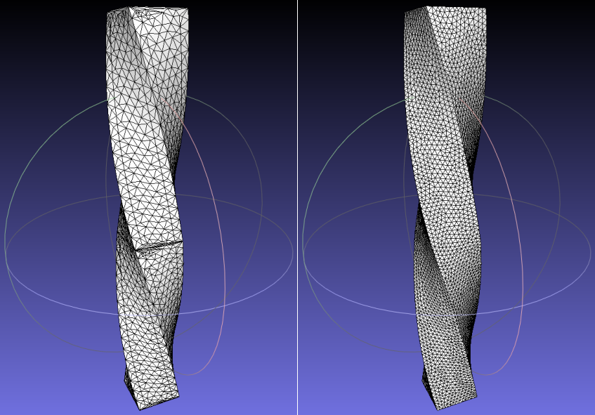
Meshes regularity (left bad, right good)

Mesh creation can be performed by any external tool such as FreeCAD or MeshLab that can generate a .stl mesh. After that, the .stl can be used to generate a .lnas file through stl2lnas.

Voxelization (experimental)

As an alternative to IBM, a body surface can be voxelized: a band of boundary-condition nodes is rasterized around the geometry and a wall BC is attached to each band node, with the wall normal snapped to the nearest cardinal direction. This is configured per body under domain.bodies.<name>.voxelization:

domain:
  bodies:
    solid-body1:
      geometry_path: "lnas/solid-body1.lnas"
      voxelization:
        run: True            # opt in to voxelization for this body
        BC: RegularizedHWBB  # band velocity BC: 'RegularizedHWBB'
        order: 0             # BC application order (less is first)
        band_radius: 1       # voxel band radius (see below)
        strict_normal: True  # raise on concave-corner nodes
        scalar_bcs:          # scalar BCs on the same band
          - scalar: temperature
            BC: ScalarRegularizedNeumann    # zero-flux (adiabatic) wall
            J_w: 0.0
          - scalar: smoke
            BC: ScalarRegularizedDirichlet  # fixed-value emission patch
            phi_w: 1.0

The band is band-only: the interior is left as dead fluid sealed behind the band (no flood fill / interior masking). The band_radius controls how many voxel layers wide the band is. The default 1 (band half-extent 1.5 dx) seals every link of the D3Q27 momentum lattice crossing the wall, including diagonals. The band width also sets the hole tolerance: STL gaps narrower than the band are healed, and two surfaces closer than the band merge into solid.

Scalar BCs on the band

scalar_bcs attaches a scalar (advection-diffusion) boundary condition to the same band nodes, independently of the velocity BC. Each entry targets one scalar field (scalar, a key under models.scalar_transports) with one of:

• ScalarRegularizedDirichlet: fixed wall value. Requires phi_w. The scalar imposes no velocity (the advection velocity comes from the fluid). Use this for a surface emission patch (a fixed-value scalar source on the band).

• ScalarRegularizedNeumann: prescribed wall flux. Requires J_w (with J_w > 0 injecting scalar, a node-source term on the band; J_w = 0 is the zero-flux adiabatic / impermeable wall).

• ScalarRegularizedRobin: convective heat-loss wall, J_w = h (phi_inf - phi_w). Requires h (transfer coefficient as a level-0 lattice velocity) and phi_inf (ambient). The wall is static.

The same cardinal-snapped normal drives both the velocity and the scalar BC. The scalar band nodes exchange cleanly across multiblock F2C/C2F: only the scalar macroscopics phi/q_neq are communicated (no momentum or force), so the exchange is force-free. Volumetric region sources are out of scope; the band attaches scalar BCs to surface nodes only.

Note

Voxelization uses cardinal-snapped wall normals with halfway / regularized halfway bounce-back for velocity and the scalar bounce-back / regularized Dirichlet / Neumann BCs for scalars. Voxel surfaces carry cardinal-snapped normals and do not support wall models. Concave-corner / multi-normal band nodes raise unless strict_normal: False. The per-node BC encoding holds up to 15 distinct (BC type x cardinal normal) combinations per field, so a planar or cylindrical surface fits comfortably while a full sphere exceeds it.

Moving bodies (experimental)

A body’s IBM transformation is normally baked into the geometry once, at load time, through domain.bodies.<name>.transformation; its Lagrangian nodes and their node-to-block relations are then fixed for the whole run. To let a body move during the simulation, set movable: True and supply a runtime transformation:

domain:
  bodies:
    solid-body1:
      geometry_path: "lnas/solid-body1.lnas"
      movable: True               # enable runtime motion for this body
      runtime_transformation:     # current pose, relative to the loaded one
        fixed_point: [0, 0, 0]
        rotation: [0, 0, 0]       # radians
        scale: [1.0, 1.0, 1.0]
        translation: [0.0, 0.0, 0.0]

runtime_transformation is a per-body 4x4 affine transform (same fields as transformation) applied to the nodes’ positions and normals relative to the loaded pose, distinct from the load-time transformation. The Lagrangian nodes are never moved in memory: the matrix is stored as body state and the IBM kernels apply it to each node’s reference position and normal at read time. The kernels also re-resolve, on the GPU, which block now holds each moved node - a short walk over same-level block neighbours from the node’s setup-time block - so no node-to-block mapping is recomputed on the host and no index buffer is re-uploaded. The only per-step host work is uploading the small 4x4 matrix; that happens before the first interpolation/spread of each step, so the kernels keep reading and writing the correct block as the body moves. Static bodies (movable: False, the default) are untouched and follow the original fixed path, with no transform applied in the generated kernels.

Prescribed motion

A static runtime_transformation is a one-shot reposition. To actually move the body over time, give it a motion time series instead - a list of keyframes pairing a level-0 time step with the body pose at that instant:

domain:
  bodies:
    solid-body1:
      geometry_path: "lnas/solid-body1.lnas"
      motion:                      # implies movable
        keyframes:
          - time: 0                # level-0 step
            transformation:
              translation: [0.0, 0.0, 0.0]
          - time: 5000
            transformation:
              translation: [25.0, 0.0, 0.0]   # 25 nodes over 5000 steps

The pose at a given level-0 time is interpolated between the bracketing keyframes (clamped to the first/last keyframe outside the range); all keyframe times are in level-0 steps. Setting motion implies movable (you need not set both). Translation, scale and fixed point interpolate linearly in time, and rotation follows a quaternion slerp, so the body rotates along a true rotation arc between keyframes at any angular separation (not a sheared, shrunk blend of rotation matrices).

The pose is evaluated only at level-0 steps. To keep finer refinement levels from seeing the body jump once per coarse step, the inner sub-steps within a coarse step linearly interpolate between the previous and current level-0 pose, so the body moves a bit per inner time step.

Because the body moves, the IBM no-slip condition is not “match a still wall” but “match the moving boundary”: the target velocity at each node is the boundary point velocity dx/dt. It is the per-coarse-step displacement of the node (current pose minus previous pose) over one level-0 step - constant across the coarse step for a linear motion - computed in-kernel from the body’s matrix state. A body with a constant pose has zero such velocity and reduces to ordinary no-slip. The displacement is taken in level-0 units; lattice velocity is level-independent, so the same value applies at every refinement level.

This is the basis for moving bodies and fluid-structure interaction: it provides the transformation plumbing, the dynamic node-to-block reassignment, the moving-boundary velocity, and a prescribed (keyframe) motion driver. A node stays on a single refinement level (it may not change level).

Because a moving node can enter a block that was not in the body’s original affected set - and that block would otherwise have no IBM force buffer, silently dropping the spread force - moving-body cases should also enable, on the body’s IBM config (models.IBM.body_cfgs.<cfg>):

models:
  IBM:
    body_cfgs:
      moving_cfg:
        allocate_force_all_blocks: True   # force buffers on every block

allocate_force_all_blocks allocates the IBM force buffers and runs the force processing on every runnable block instead of only the precomputed affected set. It uses more memory, so it is off by default and meant to be turned on for movable bodies.

Data extraction

It’s very common to extract data from a body, such as \(\rho\) for pressure calculation afterwards. This can be done by specifying bodies for extraction in data.series.series_name.bodies field.

It’s important to notice that the extraction is done using the resolution from the original mesh. The original vertices and triangles from the original .lnas are the ones used to extract data from the body (considering all bodies transformations and such).

Important

Make sure that your mesh has the desired spatial resolution for data extraction. If the mesh is more refined than required, or less refined, it should be updated for use.

Another capability is to extract data from a surface. It’s possible to specify a probe using a body as body_name.surface_name to consider only the triangles from a .lnas surface.