Introduction

Welcome to the Nassu LBM solver user guide. Nassu is the CFD engine behind the AeroSim digital wind tunnel software, built to run wind flow simulations at high performance on GPUs.

Nassu solves fluid flow with the lattice-Boltzmann method (LBM), runs natively on NVIDIA GPUs (CUDA), and is tuned for memory efficiency so that large wind engineering domains fit on a single card. Its guiding philosophy is simple: you don’t have to write a single line of code to run your simulation. You describe the simulation in a single configuration file, and Nassu does the rest.

Important

This user guide is focused on the Nassu solver and its internals. For our web interface, check out the AeroSim documentation.

Who this guide is for

This guide is written for engineers and researchers who want to run computational wind engineering (CWE) simulations: wind loads on buildings, pedestrian wind comfort, pollutant dispersion, terrain and urban flows, and external aerodynamics in general. We assume you are comfortable with the basics of fluid mechanics. You do not need prior experience with the lattice-Boltzmann method or with GPU programming.

Tip

If you are not yet familiar with CFD or LBM, the textbook by Kruger et al. (2016), The Lattice Boltzmann Method: Principles and Practice, is the recommended introduction and is referenced throughout the theory chapters.

What you will learn, and in what order

The user guide is a guided path. We recommend following it in order the first time:

1. Introduction (this page): what Nassu is, why LBM-LES, and the no-code philosophy.

2. Technologies: the Python + CUDA architecture and how Nassu generates specialised kernels for each simulation.

3. Installation and usage: install Nassu and run your first simulation from the command line with nassu run.

4. Configuring simulations: the heart of the guide. How the .yaml configuration file is structured and how to describe a domain, its bodies, the output you want, and the numerical models.

5. Post-processing: read and analyse the fields and time series the solver writes.

By the end you should be able to take a wind engineering problem, write a configuration file for it, run the simulation, and inspect the results, without writing any code.

What is CFD?

The acronym CFD stands for Computational Fluid Dynamics, the area of knowledge that studies and develops methodologies to numerically solve transport equations such as Navier-Stokes Equations (NSE).

The application of CFD extends from biological systems in hemodynamics, aerodynamics of most varied objects, plastic extrusion in industry, to visual effects in games and movies.

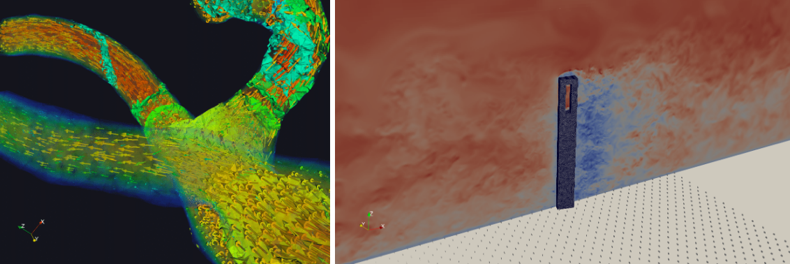
CFD examples in hemodynamics and aerodynamics

Many methods that numerically solve the NSE are available, when dealing with turbulent flows the most usual are RANS, LES and DNS:

CFD methodologies to solve turbulent flows

The Reynolds-Averaged-Navier-Stokes (RANS) solves the time-averaged NSE and returns the average properties of the flow. RANS is the most popular CFD method for turbulence due to its low computational cost. However, since in RANS the transient features of the flow are not captured, the method should be applied only to problems in which peak values are not important, which is not the case for wind pressure analysis.

At the other extreme, a Direct Numerical Simulation (DNS) explicitly solves NSE for a given \(\Delta t\) and \(\Delta x\). Great accuracy can be obtained with DNS, however its computational cost is overwhelming for turbulent flow simulations at high Reynolds numbers. Since the method has to capture all turbulent scales to properly reproduce the flow, it requires very fine temporal and spatial resolutions which leads to prohibitive computational costs.

As alternative, Large Eddy Simulations (LES) can be used to satisfactory capture transient aspects of a flow with a viable computational cost. In this methodology, the flow large scales are explicitly solved while the smaller are modelled:

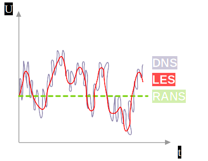
Representation of LES filtering for a velocity signal

As a result, the macroscopic signals in LES simulations will be smoothed and approach from DNS as spatial and temporal resolutions are increased.

Note

Despite its cost being inferior to DNS, the use of LES for engineering problems is also very computationally demanding, and has only become achievable recently due to constant evolution of computational processing technologies.

CFD as wind engineering tool

In wind engineering many problems can be approached using CFD when an adequate methodology and setup are adopted. In wind tunnel experiments, the pressure fluctuations on the surface of a solid body are measured with a high frequency in order to capture the extreme events that the structure eventually will be subjected to.

To achieve similar results through CFD it is necessary to adopt a method that is transient, and therefore can capture the pressure fluctuations. Wind tunnel experiments for structural design usually occur at a Reynolds numbers above \(10^{5}\), which means that the grid resolution required to represent the small turbulence scales with a DNS would be extremely high and impracticable for most computational resources available.

Hence the usual approach for such problems is LES, which can satisfactorily capture the flow statistical behavior (average, variance, kurtosis, and skewness), when a proper setup with adequate boundary conditions, grid refinement and placement of obstacles is estabilished:

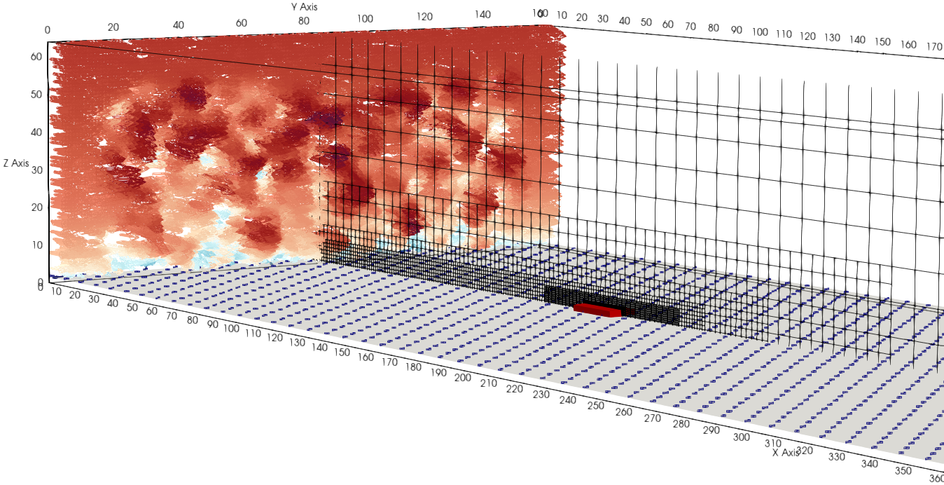
Example of LES wind tunnel setup for a low rise building

LBM to solve NSE

As previously stated, the computational cost for LES is still very high. In most LES environments a wind tunnel simulation with adequate resolution and sufficient time interval simulated for statistical analysis would require several days of computing time. This is mostly due to the fact that most LES solvers are based on finite volume methods (FVM). To address the same problem more efficiently, we adopt an alternative paradigm to solve the NSE, which is the lattice-Boltzmann method (LBM).

The LBM is developed from numerical discretization of Boltzmann equation, a partial differential equation (PDE), resulting in the lattice-Boltzmann equation (LBE). Through incompressible assumption, it can be shown that the LBE returns the NSE and hence by solving the LBE, one is solving the NSE from an alternative approach.

The main advantage of the LBM is that its operations occur mostly locally, with only the direct transcription of data series between neighboor nodes. This characteristic makes the method highly suitable for high performance parallel processing in GPU environments.

Features and performance

As the LBM only solves for the flow evolution, some other features are still required to properly represent a wind tunnel simulation. In Nassu, some of the features are:

• Complex shaped bodies and terrain are represented in computational domain with immersed boundary method (IBM)

• A turbulent inlet boundary is implemented with synthetic eddy method (SEM)

• Multigrid resolution is adopted near solid bodies

Among other features to enable the capabilities to solve complex aerodynamics problems.

The coupling between LBM and any feature affects the simulation performance overall. The operations related to these features are therefore optimized in the solver.

Nassu is able to execute wind tunnel simulations with more than 100M nodes overnight.

Important

A well known bottleneck found in most LBM developments is its memory demand. For that matter, we adopt a macroscopics collision based formulation of the LBM, that eliminates the necessity of saving several population variables for each domain node.

The no-code philosophy

All of these capabilities (the domain, bodies, refinement, turbulent inlet, boundary conditions, output, and numerical models) are selected and tuned through a single .yaml configuration file. You never edit solver source code to set up a case. This keeps simulations reproducible, easy to share (you can send a single file to a colleague or to a remote server), and quick to vary: changing a velocity, a domain size, or a refinement level is a one-line edit.

The next chapters take you from installing Nassu to writing that configuration file yourself.

Next steps

Continue to Technologies to understand the architecture, or jump straight to Installation and usage to set up Nassu and run your first simulation. When you are ready to build your own case, the Configuring simulations chapter is where the real work happens.