
 AeroSim Docs
Boundary Conditions
The boundary conditions (BCs) must be configured in order to run a simulation. The computational domain is a parallelepiped as illustrated below:
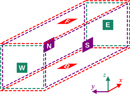
Computational domain
The BCs are defined for each plane in the models.BC field.
The example below, shows a basic wind tunnel setup with a uniform inlet inflow:
    models:
      BC:
        periodic_dims: [false, true, false]
        BC_map:
          - pos: W
            BC: UniformFlow
            wall_normal: W
            order: 2
            params:
              rho: 1.0
              ux: 0.05
              uy: 0
              uz: 0
          - pos: E
            BC: RegularizedNeumannOutlet
            wall_normal: E
            order: 2
            params:
              rho: 1.0
          - pos: F
            BC: Neumann
            wall_normal: F
            order: 1
          - pos: B
            BC: RegularizedHWBB
            wall_normal: B
            order: 1
Note
Each BC_map entry keeps its structural keys (pos, system, BC, wall_normal, order) at the top level and gathers the BC-specific parameters under a nested params: field, validated at parse time against the selected BC. The entry is extra="forbid", so a misspelled or misplaced key is rejected on load. BCs that take no parameters (such as Neumann, RegularizedHWBB, RegularizedNeumannSlip and HWBB) omit params: entirely.
If periodicity is set true for a certain direction, it does not require definition of a BC. The order determines which BC will overwrite the other at edges and corners of computational domain.
Important
It’s recommended to execute the lateral boundaries first, then top/floor, and inlet/outlet.
It’s also possible to define a BC for edges as shown below:
    models:
      BC:
        BC_map:
          - pos: NW
            BC: Neumann
            wall_normal: W
            order: 3
The wall_normal determines the offset direction to perform certain BCs and can only be defined for the domain face boundaries.
Moving wall
A wall translating at a prescribed velocity uses RegularizedVelocityWall (the
moment-based moving wall). It imposes the wall velocity, treats the wall density
according to rho_wall, and reconstructs the rate-of-strain from the wall-normal
finite difference - the no-slip RegularizedHWBB is the zero-velocity case of the
same closure. The wall velocity components are required:
    models:
      BC:
        BC_map:
          - pos: N
            BC: RegularizedVelocityWall
            wall_normal: N
            order: 1
            params:
              ux: 0.02
              uy: 0
              uz: 0
Wall density treatment (rho_wall)
Both wall closures (the no-slip RegularizedHWBB and the moving
RegularizedVelocityWall) accept an optional rho_wall that selects how the wall
density is set:
Omitted (default): zero-normal-gradient. The wall density is extrapolated from the interior wall-normal neighbour (
rho = rho_d1). This is the physically correct closure for a no-slip wall, where the wall-normal pressure gradient is negligible, and for recirculating flows (for example a lid-driven cavity) where the wall pressure varies along the wall. It is the recommended default for solid walls.Supplied: fixed density. Giving a positive
rho_wallfixes the wall density to that constant (the wall pressure is held uniform). Use this only for outlet-like or genuinely uniform-pressure walls (for example Couette / Poiseuille channels); fixing the density on a wall with a varying pressure field degrades accuracy.
The choice is made per wall node, so different walls of the same type may mix the
two treatments. To fix the density, add rho_wall to the BC entry:
          - pos: N
            BC: RegularizedVelocityWall
            wall_normal: N
            order: 1
            params:
              ux: 0.02
              uy: 0
              uz: 0
              rho_wall: 1.0
Predicate-based BC regions
Besides the cardinal aliases (N, S, E, W, F, B and their edge/corner
combinations), the pos field accepts a boolean predicate over the node
coordinates x, y, z. This selects every node whose coordinate satisfies the
expression, allowing interior walls, slabs, cuboids, pipes, spheres and any
boolean composition of those without an STL/IBM geometry.
    models:
      BC:
        BC_map:
          # Interior axis-aligned baffle (a cuboid slab cutting the domain)
          - pos: "(x >= 14) & (x <= 17) & (8 <= y) & (y <= 24)"
            BC: RegularizedHWBB
            wall_normal: E
            order: 2
          # A circular pipe wall region
          - pos: "(x - 50)**2 + (y - 50)**2 >= 40**2"
            BC: RegularizedHWBB
            wall_normal: E
            order: 1
The grammar supports the coordinate symbols x, y, z, real constants, the
operators + - * / and integer powers (** or ^), the comparisons
<, <=, >, >=, ==, !=, and the boolean operators and/&, or/|,
not/~. The expression must evaluate to a boolean (a comparison or a boolean
combination of comparisons). Transcendental functions (sin, log, …) and
non-integer powers are outside the grammar and raise a configuration error.
The coordinates are the global node coordinates of the domain; on a single-level
domain these are the lattice-node indices. A cardinal alias is exactly
equivalent to a predicate (N is y >= Ny - 1, S is y <= 0, and so on),
so existing configurations keep working unchanged.
On a refined domain the predicate is evaluated in those same global level-0 lattice coordinates on every block, whatever its refinement level, so a region overlapping a refined block selects that block’s nodes at the finer spacing. The selected node count therefore follows the local spacing, and a region straddling a refinement interface is denser on the fine side.
The same pos grammar applies to the per-scalar boundary conditions under
models.scalar_transports.<name>.BC.BC_map, so an emitting footprint on the
ground, a road line or any interior surface is expressed for a scalar exactly as
it is for the fluid:
    models:
      scalar_transports:
        pollutant:
          BC:
            BC_map:
              # Fixed concentration over a ground footprint
              - pos: "(z <= 0) & (x >= 120) & (x <= 180) & (y >= 40) & (y <= 90)"
                BC: ScalarRegularizedDirichlet
                wall_normal: B
                order: 1
                params:
                  phi_w: 1.0
Important
The wall_normal is the outward cardinal direction of the wall and is stated
explicitly on the entry. It is never inferred from pos: a predicate region takes
the same explicit cardinal normal a cardinal alias does. Every scheme that
reconstructs along the wall normal requires it (only UniformFlow and
ScalarUniformInlet do not), and an entry that omits it is rejected at config
load.
Floating/curved regions defined by a single comparison (x^2 + y^2 < R^2, a
tilted half-space, …) additionally carry a true continuous unit normal derived
analytically from the predicate gradient and stored per node (snorm int8 per
component) in a global array, exported with the wall-normal map. The
continuous-normal array is allocated only when a floating region needs it.
Planes, lines and points: the thickness convention
A predicate is evaluated once per node, so a geometry with zero measure - a plane, a line, a point - contains no node except by accident and has to be thickened before it selects anything. Nassu uses one convention everywhere:
Authored extents are closed. Thickened (zero-measure) directions are half-open and exactly one baseline cell wide.
h is the level-0 (baseline) cell size expressed in the frame the predicate is
written in. In lattice coordinates that number is exactly 1, because a
predicate sees the global node coordinate block.pos + index * block.interval
with interval = 0.5 ** level. A predicate written in a domain.systems frame
(metres, say) uses the baseline cell size in that frame.
Geometry |
Predicate |
Endpoints |
|---|---|---|
Point at |
|
half-open on every axis |
Plane, normal |
|
half-open on the normal, closed in-plane |
Line, dominant axis |
|
closed along the segment, half-open transverse |
Box |
|
closed on every face |
Two properties follow, and they are the reason for the shapes above:
A half-open interval of width exactly
htiles the axis, so it selects exactly one node layer wherever the geometry falls relative to the node grid. A closed interval of the same width selects two layers whenever a node plane lands on a face.The thickness is the baseline cell, not the local refined cell. The grammar has only
x,yandz, so a level-aware width cannot be written. Inside a refinement of levelLa thickened direction holds2**Lnode layers; sizing it to the finest resolution instead would select nothing at all in unrefined space.
The line form is a discrete line rather than a tube of radius h/2: it selects
exactly one node per lattice step of its dominant axis, and it is never empty. An
isotropic tube of radius h/2 is empty for an axis-parallel line offset half a
cell on both transverse axes, which sits sqrt(2)/2 * h from every node.
Placing a region with a typed shape
The predicate above can also be named as a shape: pos takes a kind-tagged
mapping as readily as it takes a string. Both spell the same region and select the
same nodes, because the shape is lowered to the equivalent predicate at config
load, following the thickness convention above, so the convention has one owner
and a client never derives it.
The kinds and their fields, the same vocabulary an export probe uses:
|
Fields |
Region |
|---|---|---|
|
|
the one node whose cell contains the point |
|
|
one node per listed point |
|
|
the segment, one node per step of its dominant axis |
|
|
one node layer, optionally bounded in-plane |
|
|
the closed axis-aligned extent |
|
|
the same box, named from its centre |
|
|
the closed ball |
|
|
the closed cylinder of revolution |
|
|
the predicate string itself |
    models:
      BC:
        BC_map:
          - pos: {kind: point, pos: [10, 20, 5]}
            BC: RegularizedHWBB
            wall_normal: E
            order: 1
          - pos: {kind: points, points: [[10, 20, 5], [11, 20, 5]]}
            BC: RegularizedHWBB
            wall_normal: E
            order: 1
          - pos: {kind: line, start: [10, 20, 5], end: [40, 20, 5]}
            BC: RegularizedHWBB
            wall_normal: E
            order: 1
          - pos: {kind: plane, axis: z, axis_pos: 0.0, min: [10, 10], max: [50, 50]}
            BC: RegularizedHWBB
            wall_normal: B
            order: 1
          - pos: {kind: box, start: [10, 10, 0], end: [50, 50, 20], is_abs: true}
            BC: RegularizedHWBB
            wall_normal: E
            order: 1
          - pos: {kind: sphere, center: [50, 50, 30], radius: 20}
            BC: RegularizedHWBB
            wall_normal: E
            order: 1
          - pos: {kind: cylinder, center: [50, 50, 30], radius: 10, height: 40, axis: z}
            BC: RegularizedHWBB
            wall_normal: E
            order: 1
          - pos: {kind: predicate, predicate: "(x - 50)**2 + (y - 50)**2 < 400"}
            BC: RegularizedHWBB
            wall_normal: E
            order: 1
A shape is written the way it is drawn. An extent is named by its corners; a round
shape is named by its centre and the dimensions measured from it, so a sphere
is a center and a radius, and a cylinder adds the full height (not a
half-extent) along its axis. A box takes either spelling - start/end or
center/size, the full side per axis - and exactly one of them, since they are
two names for one shape and center/size is resolved into the corner pair at
config load. The centred spelling is absolute; is_abs belongs to the corner pair.
A cylinder’s axis is its axis of revolution in the shape’s own frame, one of
x, y, z and z by default. A cylinder pointing anywhere else is that
cylinder plus a transformation, the same way a plane carries its orientation. In
a 2-D simulation a sphere is a disc, and a cylinder is a disc too - only the
out-of-plane axis is meaningful there.
A round shape is exact within the predicate grammar: a squared distance is a sum of integer powers, so nothing is thickened. A sphere smaller than a lattice cell therefore selects no node at all - a region is the set of nodes inside the authored shape, never a shape grown until it catches one.
A position’s coordinates are lattice coordinates unless the entry names a frame. Two optional fields place it, exactly as they place a refinement volume:
system, on the entry besidepos: the name of adomain.systemsframe the coordinates are written in, defaulting todomain.default_system. Rotated systems are supported. It qualifiesposin either spelling, a predicate string or a shape, and is not valid on a cardinal alias, which is an lbm-frame domain face by definition.transformation, on the shape: a rigid transform (rotation,translation,scaleaboutfixed_point) mapping the shape’s own local frame into that system.
          - pos:
              kind: plane
              axis: z
              axis_pos: 0.0
              min: [10, 10]
              max: [50, 50]
              transformation:
                rotation: [0, 0, 0.7854]
            system: site
            BC: RegularizedHWBB
            wall_normal: B
            order: 1
What the lowering leaves on the record
A shape and its frame are consumed by the lowering: pos becomes a lattice-frame
predicate and system is cleared, so the config the run writes to its output folder
describes the region as an expression rather than as the shape that was asked for.
For a shape in a rotated frame that expression is expanded algebra, unreadable at a
glance and impossible to draw.
The entry therefore keeps pos_authored, a record of what the placement said:
    pos: (-0.707106793288165*x + 0.707106793288165*y >= 0) & ...
    pos_authored:
      pos: {kind: box, start: [10.0, 10.0, 0.0], end: [50.0, 50.0, 20.0], is_abs: true}
      system: site
It is derived, not an input: it is filled in when the lowering rewrites pos, no
solver path reads it, and a position that survives the pass unchanged - a cardinal
alias, or a predicate already written in the lattice frame - records nothing,
because pos is then its own source. Re-validating an exported config keeps the
original record rather than replacing it with the lowered predicate.
The frame is baked into the lowered predicate, and the thickness follows it: a
thickened direction is one lattice cell wide whatever units the shape is
authored in. A frame that scales the axes differently has no single cell size and
is rejected for the thickened kinds (point, points, line, plane); box,
sphere, cylinder and predicate thicken nothing and accept it.
Only is_abs: true boxes can carry a frame. A relative box (is_abs: false) is a
fraction of the domain size, like a relative refinement volume, and has no
physical frame.
A box names a region rather than a direction, so its corners may be written in
either order - start: [10, 5, 5], end: [2, 1, 1] is the same box as its reverse,
and the pair is ordered per axis when the config loads. The same holds for a
plane’s min/max and for every volume (a refinement volume, an export target).
A pair that is equal on some axis is still rejected: that is a zero-thickness
region, a different mistake from writing the corners backwards. A line is
directed and keeps the order it was written in.
The same shape, in an export probe
A shape is written the same way wherever it appears. The line a BC is placed on
and the line an export samples along carry the same start and end; a plane is
axis / axis_pos / min / max on both sides; a box is start / end /
is_abs whether it is a pos, a refinement volume or an export target. system
means the same thing everywhere, and transformation is the same rigid transform.
What differs is not the specification but what is done with it:
A placement shape ( |
An export probe ( |
|
|---|---|---|
Answers |
which nodes are in the region |
where to take samples |
Produces |
a node predicate, thickened by the convention above |
a point cloud at |
Extra field |
none |
|
So dist is a probe field only: a probe generates sample points and needs a
spacing between them, while a placement shape takes the nodes the lattice already
has. A pos given a dist is rejected, saying so.
The reverse is equally deliberate: a probe has no thickness convention, because it
never selects nodes. A plane probe with dist: 0.5 samples a grid on the plane
regardless of where the nodes sit; a kind: plane placement selects exactly the
one node layer inside a slab one cell thick.
Volumetric (region) boundary conditions
Surface BCs act on the domain faces; a volumetric boundary condition acts on
every fluid node inside a region of the domain. Volumetric regions are configured
under models.volumetric_regions, a mapping whose keys name the regions, and each
region is placed by the same pos a surface BC takes, so a cuboid is
(x >= xa) & (x <= xb) & .... Region nodes are flagged on the lattice bitmap (a
reserved per-node bit, no extra memory), and the volumetric term is applied in the
LBM bulk only where the flag is set.
A volumetric region applies a porous-medium momentum sink to the fluid on region nodes, combining two body-force contributions:
a linear (Darcy) term
F[a] = -porous_alpha * u[a], damping momentum proportionally to the local velocity (e.g. a porous block at the outlet to suppress pressure waves and near-outlet velocity);a quadratic (Forchheimer / canopy) term
F[a] = -porous_beta * |u| * u[a], modelling pressure-decay / canopy drag whose resistance grows with the square of the speed (e.g. a forest-canopy momentum sink).
models:
  volumetric_regions:
    # Linear Darcy outlet sponge (beta omitted -> 0).
    outlet_sponge:
      pos: "(x >= 480) & (x <= 500)"
      porous_alpha: 0.2
      porous_beta: 0.05
    # Quadratic canopy drag region: a different medium with its own
    # coefficients, placed as a typed shape instead of a predicate.
    canopy:
      pos: {kind: box, start: [100, 0, 0], end: [200, 500, 20]}
      porous_alpha: 0.01
      porous_beta: 0.05
    # A porous ground layer, named by the cardinal alias for the B face.
    ground:
      pos: B
      porous_alpha: 0.2
A volumetric region takes every spelling of pos a surface BC takes - a cardinal
alias, a predicate or a typed shape - with the same kinds and the same system /
transformation envelope. A cardinal alias on a volume names the node layer at
that domain face.
One region, several shapes
One medium usually occupies several disjoint pieces of the domain: a row of trees,
a bank of burners, a handful of gravel beds. A region’s pos therefore also takes
a set of shapes, listed under the plural of their kind (spheres, boxes,
cylinders, planes, lines, points) plus predicates. The kind tag is
implied by the list key and is not written, exactly as an export target’s entities
do not repeat theirs.
models:
  volumetric_regions:
    tree_row:
      # Written once, for every shape below.
      porous_alpha: 0.0
      porous_beta: 0.928
      system: terrain
      pos:
        spheres:
          - {center: [200, 72, 8], radius: 6}
          - {center: [240, 72, 8], radius: 6}
          # This crown's centre comes from another survey.
          - {center: [12, 4, 8], radius: 6, system: tower_local}
        cylinders:
          - center: [240, 72, 4]
            radius: 0.6
            height: 8
            axis: z
            transformation: {rotation: [0.26, 0, 0], fixed_point: [240, 72, 0]}
        predicates:
          - "(z >= 0) & (z <= 1)"
The shapes are lowered individually and OR-ed into one region, so the set is a single entry of the list wherever a region is indexed: one region index, one row of the coefficient table, one node of the per-node region map. Twelve crowns of one medium cost what one region costs.
The frame follows the shapes. The region’s system is the frame every shape it
lists defaults to, and a shape naming its own overrides it - a region whose
reference points (a sphere’s center, a box’s corners) come from two surveys is
still one region. transformation stays per shape, mapping that shape’s own local
frame into the system it is written in. A predicates entry is the predicate
string itself: it is qualified by the resolved system like any other predicate and
takes no transformation, so a hand-written predicate that needs a rigid transform
is written as a single pos with kind: predicate.
Each transported field’s source_regions takes the same set spelling, with the
emission rate written once for every shape the region covers.
Both porous_alpha and porous_beta (>= 0, lattice units) are compile-time
constants baked into the generated kernel. Each region is its own medium with its
own pair, so an outlet sponge and a canopy coexist in one domain. porous_beta
defaults to 0 (linear-only).
Note
Every mapping of volumetric regions - models.volumetric_regions and each
transported field’s source_regions - resolves an overlap the same way: a node
inside several regions belongs to the region declared last (the key order).
The shapes of a single region are one region and never overlap each other.
That is a different mechanism from a BC’s order, which is the order in which
boundary conditions are applied (an order-1 BC overwrites an order-0 one on a
node they share). A region mapping has no order: its precedence is its
declaration order.
Turbulent inflow
In many simulations it’s desired to use a turbulent inflow.
This is configured under models.BC.inlet_turbulence, which selects an inlet turbulence generator by its type field.
type: sem: the synthetic eddy method (SEM).type: podfs: the proper orthogonal decomposition Fourier series (PODFS) method.
The turbulent inflow is limited to the W boundary.
Synthetic eddy method (SEM)
A simulation set to use SEM as inlet will have the following aspect:
    models:
      BC:
        periodic_dims: [false, false, false]
        BC_map:
          - pos: E
            BC: RegularizedNeumannOutlet
            wall_normal: E
            order: 2
            params:
              rho: 1.0
          - pos: F
            BC: Neumann
            wall_normal: F
            order: 1
          - pos: B
            BC: RegularizedHWBB
            wall_normal: B
            order: 1
          - pos: N
            BC: Neumann
            wall_normal: N
            order: 0
          - pos: S
            BC: Neumann
            wall_normal: S
            order: 0
        inlet_turbulence:
          type: sem
          eddies:
            lengthscale: {x: 14, y: 14, z: 14}
            eddies_vol_density: 10
            seed_rand: 0
            domain_limits_yz:
              start: [-14, -14]
              end: [174, 78]
          profile:
            csv_profile_data: "../SEM/vprofile.csv"
            z_offset: 3.6
            K: 1
            length_mul: 1
            vel_mul: 1
The .csv file for profile.csv_profile_data describe the velocity profile and its stress tensor.
It must contain the headers: z,ux,Rxx,Ryy,Rzz,Rxz,Rxy,Ryz
z: Height for given valuesux: Average velocity for the given heightRxx,Ryy,Rzz,Rxz,Rxy,Ryz: Reynolds stress tensor for given height
Note
The values in between are found using linear interpolation, or constant extrapolation for values higher or lower than z max, min.
Density of eddies is given by eddies_vol_density, which is the density of eddies by volume, so for 10 it means that every SEM domain node will have 10 eddies affecting it in average.
The randomization of eddies generation can be controlled using the seed_rand, so when using the same seed_rand and other configurations the same series of eddies are generated (making it possible to reproduce the same inlet multiple times).
The height of velocity profile can be adjusted with profile.z_offset. The profile is a function of height \(z\) only; the inlet is homogeneous in the lateral (\(y\)) direction.
Eddies are seeded only inside eddies.domain_limits_yz; outside it the inlet carries the mean velocity alone. The box is usually inset from the inlet face by the eddy lengthscale, so that no eddy straddles the border, which makes its corners a function of the domain size and of eddies.lengthscale rather than free choices - the validation cases write them as !math on the domain dimensions for exactly that reason.
Note
domain_limits_yz is written low-to-high on each axis: start below end in both \(y\) and \(z\). An inverted axis is rejected rather than reordered, because a derived corner pair that comes out inverted reports an impossible region - the inset consumed the whole edge - and reordering it would hand the solver a band nobody asked for. It happens when the domain is narrower than twice the inset on that axis: widen the domain there, raise the resolution, or lower the lengthscale on that axis.
Note
Examples can be found in nassu/fixture/SEM/ folder.
Proper orthogonal decomposition Fourier series (PODFS)
PODFS is a data-driven inlet generator: it builds a compact temporal basis from a turbulent precursor and replays it at the inlet through a Fourier series, so the injected field is continuous, periodic and independent of the solver time step. The theory is described in the PODFS theory page.
PODFS uses a two-step, load-only workflow. The plane-sampling to POD transform is a separate offline process; the solver only loads a finished basis file and replays it.
Step 1 - build the basis offline. Run nassu podfs-build on a small build-spec YAML (a standalone file, not a .nassu.yaml sim config) that describes the precursor source and the build parameters. It writes a single, self-describing basis file (HDF5) holding the mean profile, the POD modes, the Fourier coefficients, the analysis-grid coordinates, and an optional calibrated high-frequency supplement:
uv run nassu podfs-build my_case.podfs-build.yaml
A build-spec describes either a synthetic precursor (synthetic:) or a recorded plane-series export (plane: pointing at an .xdmf), plus the build knobs:
synthetic:
  grid_shape: [16, 24]      # structured (n_a, n_b) analysis grid
  extent: [12.0, 12.0]      # physical span (extent_a, extent_b); a -> y, b -> z
  n_snapshots: 256
  dt_s: 1.0
  mean_profile: log         # the mean ux(z) baked into the basis file
  mean_amplitude: 1.0
  modes:
    - { kind: sin_a, frequency: 0.1, wavenumber_a: 1.0, wavenumber_b: 1.0, amplitude: 1.0 }
  target_variance: { ux: 0.04, uy: 0.01, uz: 0.01 }
  seed: 0
energy_target: 0.99         # cumulative POD energy retained (or set n_modes)
high_freq: false            # calibrate and store the high-frequency supplement
supplement_seed: 0
weight:                     # optional weighted POD (omit for the uniform POD)
  z: { kind: variance, eps: 0.05 }                  # data-driven 1/variance along z
  y: { kind: gaussian, sigma: 0.3, scale: 80 }      # parametric bell along y
out_path: ./basis.h5
All POD decisions (energy target, mode and harmonic counts, the mean profile, the supplement, and the weighting) are made here, offline, and frozen into the file.
Weighted POD (weight). By default the POD is energy-optimal in the uniform norm, so it allocates modes by global energy and can under-resolve the near-wall small scales. The optional weight block biases the decomposition with a per-axis separable weight \(w = w_z(z)\,w_y(y)\); each axis (z, y) independently picks its method, or is omitted to stay uniform - so you can mix, e.g. data-driven variance in z and a parametric gaussian in y:
gaussian- a 1-D bell peaking at 1 (at the ground forz, atcenter(default span mid) fory) and equal tosigmaatscalefrom the peak (\(s = \text{scale}/\sqrt{2\ln(1/\sigma)}\), no floor - beyondscaleit keeps decaying, so setscaleto where you want the weight to besigma, typically the domain extent).variance- the self-tuning \(1/\text{variance}\) profile along that axis (the per-point fluctuation variance averaged over the other axis), regularised byeps(a fraction of the mean variance, capping the boost at \(\sim 1/\texttt{eps}\)) and optionallymax_ratio. This targets uniform relative fidelity - it boosts wherever the energy is low - rather than a geometric region, and which part of the axis it emphasises depends on the data (inspect the storedweight.png). It tends to spike on the first near-wall node where the absolute variance collapses with the mean velocity.ti- proportional to the streamwise turbulence intensity \(I_u = \sqrt{\langle u_x'^2\rangle}/|U_x|\) along that axis (epsregularises the mean velocity near the wall). A smoother, physically meaningful emphasis on the high-relative-turbulence region thanvariance(the \(\sqrt{}\) compresses the dynamic range so it does not spike on the first node).
The leading modes then resolve the emphasised region better at a given mode count. This is purely an offline build choice - the basis-file format and the runtime injection are unchanged.
The chosen weight is stored in the basis file and, when a weight block is given, nassu podfs-build writes a <basis>.weight.png (the \(w(y,z)\) heatmap plus its profiles through the peak) so the emphasis can be inspected and tuned.
Step 2 - run the case, load-only. The runtime config just points basis_path at the prebuilt file and sets the unit/replay knobs:
    models:
      BC:
        inlet_turbulence:
          type: podfs
          basis_path: "../PODFS/basis.h5"
          vel_mul: 1.0
          time_rescale: 1.0
          high_freq: true
The mean velocity profile now lives inside the basis file (no runtime CSV). The unit conversion uses two independent linear knobs: vel_mul rescales the whole velocity (mean and fluctuation together, preserving the turbulence-intensity ratio), and time_rescale maps the basis temporal axis onto the solver clock (effective period \(T_\mathrm{eff} = T / \texttt{time\_rescale}\)). high_freq (default true) uses the high-frequency supplement stored in the basis file when present; it has no effect when the basis carries none.
Spatial placement (spatial). The PODFS basis lives on its own structured analysis grid, decoupled from the inlet lattice. That grid (grid_shape, extent) is chosen at build time and stored with the basis coordinates. At runtime the mean and each POD mode are bilinearly resampled from the analysis grid onto the inlet nodes of every refinement level, through an explicit affine placement so the precursor may differ from the inlet in resolution, extent, and spatial scale (for example a 12 m precursor onto a 10 m inlet). The placement is symmetric in y and grounded in z:
          spatial:
            y_center: 80.0   # span centreline (default: inlet mid-width)
            y_scale: 1.0     # spanwise stretch of the basis width about y_center
            z_offset: 5.01   # ground level (default: basis recorded z-bottom)
            z_scale: 1.0     # vertical stretch of the basis height from z_offset
The basis width maps symmetrically about y_center (so a span mismatch displaces both edges equally instead of piling deviation onto one edge, matching the usual centred refinement), and the basis height maps upward from z_offset (the ground). Below z_offset both the mean and the fluctuation are zero (treated as below-ground); outside the lateral span the mean profile still applies. When spatial is omitted the precursor is placed at its native span, centred on the inlet mid-width and grounded at its recorded height (no distortion). PODFS supports multiple refinement levels at the inlet: every level receives its own resampled modes and is injected at its own physical time.
Load-time options. A rich basis can be built once and replayed as a cheaper subset, without rebuilding the POD. The mode count is cropped by either count or energy: n_modes keeps the first N energy-ranked modes, or energy_crop (0-1) keeps the fewest modes reaching that cumulative energy fraction (the two are mutually exclusive). n_harmonics keeps the DC term plus the first K Fourier harmonics. All clamp to what the basis holds; omit to use everything. This makes mode-count / energy sensitivity sweeps a config change rather than a rebuild. The stored mean can also be replaced at runtime with mean_profile (a CSV with columns z, ux, plus z_offset/length_mul); vel_mul then scales the override along with the fluctuation.
Inspecting the basis. nassu podfs-build writes two companions alongside the basis file. <basis>.modes.xdmf opens in ParaView - scrub the time slider to step through the spatial structure of each POD mode (frame 0 is the mean, frames 1..N are the modes), colouring by ux/uy/uz. <basis>.energy.png shows the per-mode energy (log scale) and the cumulative-energy curve with the 90/95/99% crossings marked, so you can pick a sensible n_modes / energy_crop for the run.
Important
For more details check the models documentation.