Poiseuille Channel (Multilevel)

In this simulation, the multilevel approach is tested to check the macroscopics continuity when passing through different levels and when applied at boundary regions of the computational domain.

from nassu.cfg.model import ConfigScheme

filename = "tests/validation/cases/02_poiseuille_channel_flow.nassu.yaml"

sim_cfgs = ConfigScheme.sim_cfgs_from_file_dct(filename)

In this case, a small value for the relaxation time \(\tau\) was adopted. Since the aim is to check possible discontinuities in the multilevel formulation, less stable values of \(\tau\) could highlight implementation issues.

sim_cfg = next(
    sim_cfg
    for (name, _), sim_cfg in sim_cfgs.items()
    if name == "velocityNeumannPoiseuilleChannelMultilevel"
)

Extract data from multiblock data from output file of macrs export

import numpy as np
from vtk.util.numpy_support import vtk_to_numpy
from tests.validation.notebooks import common

extracted_data = {}
array_to_extract = "ux"

export_instantaneous_cfg = sim_cfg.output.instantaneous
macr_export = export_instantaneous_cfg["default"]
time_step = macr_export.time_steps(sim_cfg.n_steps)[-1]
reader = macr_export.read_vtm_export(time_step)

p1 = [sim_cfg.domain.domain_size.x * 0.75, 0.5, 0]
p2 = [sim_cfg.domain.domain_size.x * 0.75, sim_cfg.domain.domain_size.y - 0.5, 0]
line = common.create_line(p1, p2, sim_cfg.domain.domain_size.y - 1)

# Get the points from the vtkLineSource
polyData = line.GetOutput()
points = polyData.GetPoints()

pos = np.linspace(p1, p2, sim_cfg.domain.domain_size.y)

probe_filter = common.probe_over_line(line, reader.GetOutput())

probed_data = vtk_to_numpy(probe_filter.GetOutput().GetPointData().GetArray(array_to_extract))
extracted_data[(sim_cfg.sim_id, sim_cfg.name)] = {"pos": pos, "data": probed_data}

extracted_data.keys()

dict_keys([(0, 'velocityNeumannPoiseuilleChannelMultilevel')])

Extract data from multiblock data from output file of macrs export for rho plotting

average_data = {}
array_to_extract = "rho"

for time_step in macr_export.interval.get_all_process_steps(sim_cfg.n_steps):
    reader = macr_export.read_vtm_export(time_step)

    multiblock_dataset = reader.GetOutput()
    n_blocks = multiblock_dataset.GetNumberOfBlocks()

    blocks_data = []
    for i in range(n_blocks):
        block = multiblock_dataset.GetBlock(i)
        data_array = vtk_to_numpy(block.GetCellData().GetArray(array_to_extract))
        blocks_data.append(data_array)
    multiblock_avg = np.average(np.concatenate(blocks_data).flatten())

    average_data[(sim_cfg.sim_id, sim_cfg.name, time_step)] = multiblock_avg

average_data

{(0, 'velocityNeumannPoiseuilleChannelMultilevel', 0): 1.0,
 (0, 'velocityNeumannPoiseuilleChannelMultilevel', 12000): 1.0145637,
 (0, 'velocityNeumannPoiseuilleChannelMultilevel', 24000): 1.0145637,
 (0, 'velocityNeumannPoiseuilleChannelMultilevel', 36000): 1.0145637,
 (0, 'velocityNeumannPoiseuilleChannelMultilevel', 48000): 1.0145637,
 (0, 'velocityNeumannPoiseuilleChannelMultilevel', 60000): 1.0145637,
 (0, 'velocityNeumannPoiseuilleChannelMultilevel', 64000): 1.0145637}

Extract data from multiblock data from output file of macrs export for profile plotting

profile_data = {}
array_to_extract = "ux"

time_step = macr_export.time_steps(sim_cfg.n_steps)[-1]
reader = macr_export.read_vtm_export(time_step)

# p1 = [0.5, sim_cfg.domain.domain_size.y / 2 - 0.5, bounds_z[0]]
# p2 = [sim_cfg.domain.domain_size.x - 0.5, sim_cfg.domain.domain_size.y / 2 - 0.5, bounds_z[1]]
# line = create_line(p1, p2, sim_cfg.domain.domain_size.x - 1)
p1 = [0.25, sim_cfg.domain.domain_size.y / 2, 0]
p2 = [sim_cfg.domain.domain_size.x - 0.25, sim_cfg.domain.domain_size.y / 2, 0]
line = common.create_line(p1, p2, 2 * sim_cfg.domain.domain_size.x - 1)

# Get the points from the vtkLineSource
polyData = line.GetOutput()
points = polyData.GetPoints()

pos = np.linspace(p1, p2, sim_cfg.domain.domain_size.x * 2)

probe_filter = common.probe_over_line(line, reader.GetOutput())

probed_data = vtk_to_numpy(probe_filter.GetOutput().GetPointData().GetArray(array_to_extract))
profile_data[(sim_cfg.sim_id, sim_cfg.name)] = {"pos": np.array(pos), "data": probed_data}

profile_data.keys()

dict_keys([(0, 'velocityNeumannPoiseuilleChannelMultilevel')])

Results

The velocity profile at the end of simulation is compared with the steady state analytical solution below:

Processing functions for Poiseuille Flow case

from typing import Callable


def get_poiseuille_analytical_func() -> Callable:
    """Poiseuille analytical velocity function

    Returns:
        Callable: Analytical velocity function
    """
    return lambda pos: 6 * (pos - pos**2)


def plot_analytical_poiseuille_vels(ax):
    x = np.arange(0, 1.01, 0.01)
    analytical_func = get_poiseuille_analytical_func()
    analytical_data = analytical_func(x)
    ax.plot(x, analytical_data, "--k", label="Analytical")

import matplotlib.pyplot as plt

fig, ax = plt.subplots()
fig.set_size_inches(6, 5)

style_num = ["o", "^", "s", "+", "x"]

num_data = extracted_data[(sim_cfg.sim_id, sim_cfg.name)]
num_avg_vel = np.average(num_data["data"])
position_vector = (num_data["pos"][:, 1] - 0.5) / (sim_cfg.domain.domain_size.y - 1)
ax.plot(
    position_vector,
    num_data["data"] / num_avg_vel,
    style_num[0],
    label=f"N={sim_cfg.domain.domain_size.x} (avg. {num_avg_vel:.2e})",
    fillstyle="none",
    c="k",
)

plot_analytical_poiseuille_vels(ax)
ax.set_title(
    f"Poiseuille (Multilevel)\n({sim_cfg.models.LBM.vel_set} {sim_cfg.models.LBM.coll_oper})"
)
ax.legend()
plt.show(fig)

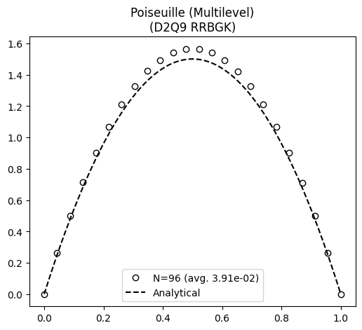
No discontinuities issues are seen through the velocity profile, indicating a satisfactory implementation.

fig, ax = plt.subplots()
fig.set_size_inches(6, 5)

plotting_data: list[float] = []
axis_data: list[int] = []

for (_, _, timestep), average_val in average_data.items():
    plotting_data.append(average_val)
    axis_data.append(timestep)

ax.plot(axis_data, plotting_data, "ok", label=f"Average {array_to_extract}", fillstyle="none")
ax.legend()
plt.show(fig)

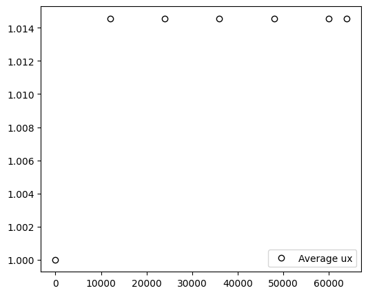
The average pressure sustains the convergence aspect exhibited in the single level simulation, though it takes longer to converge since a smaller value of \(\tau\) was adopted.

import pyvista as pv

array_to_inspect = "rho"

plotter = pv.Plotter(window_size=(800, 400))

time_step = macr_export.time_steps(sim_cfg.n_steps)[-1]
multiblock_file = macr_export.time_step_filename(time_step, ".vtm")
mesh = pv.read(multiblock_file)
mesh.set_active_scalars(array_to_inspect)
plotter.add_mesh(mesh, cmap="coolwarm")

plot_title = f"{array_to_inspect} profile Poiseuille (Multilevel)\n({sim_cfg.models.LBM.vel_set} {sim_cfg.models.LBM.coll_oper})"
plotter.add_text(plot_title, position="upper_right", font_size=18, color="black")
plotter.camera_position = [(48.0, 12.0, -192.16548199848856), (48.0, 12.0, 1.0), (0.0, -1.0, 0.0)]
plotter.camera.zoom(2)
plotter.show(jupyter_backend="static")
# plotter.show(jupyter_backend='static', cpos="xy", return_cpos=True) # Trick to get automatically the camera position

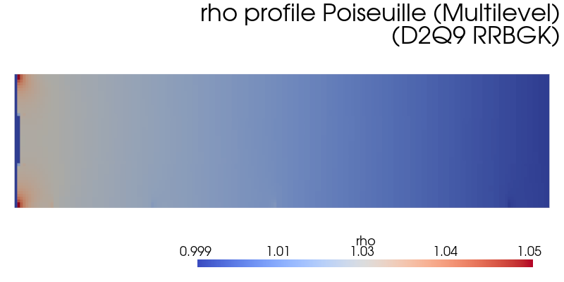
The general flow’s density profile shown above presents no visible disconuity.

fig, ax = plt.subplots()
fig.set_size_inches(6, 5)

num_data = profile_data[(sim_cfg.sim_id, sim_cfg.name)]
position_vector = (num_data["pos"][:, 0] - 0.5) / (sim_cfg.domain.domain_size.x - 1)
ax.plot(position_vector, num_data["data"], c="k")

ax.set_title(
    f"Ux profile Poiseuille (Velocity-Neumann) ({sim_cfg.models.LBM.vel_set} {sim_cfg.models.LBM.coll_oper})"
)
plt.show(fig)

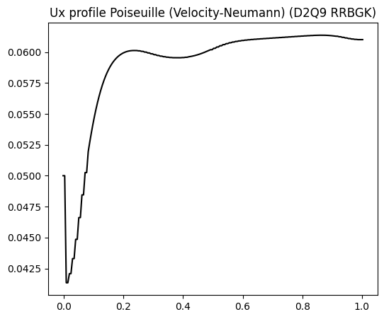
The centerline velocity has an asympotic profile. However, it would take a longer length for the velocity to completely stabilizes.

Version

sim_info = sim_cfg.output.read_info()

nassu_commit = sim_info["commit"]
nassu_version = sim_info["version"]
print("Version:", nassu_version)
print("Commit hash:", nassu_commit)

Version: 1.6.17
Commit hash: 03afae00d1166dcb73bd88413bb3cfda7b6c686c

Configuration

from IPython.display import Code

Code(filename=filename)

simulations:
  - name: periodicPoiseuilleChannel
    save_path: ./tests/validation/results/02_poiseuille_channel_flow/periodic

    n_steps: !unroll [250, 1000, 4000, 16000]

    report:
      frequency: 1000

    domain:
      domain_size:
        x: !unroll [4, 8, 16, 32]
        y: !unroll [4, 8, 16, 32]
      block_size: !unroll [4, 8, 8, 8]

    data:
      divergence: { frequency: 50 }
      instantaneous:
        default: { interval: { frequency: 0 }, macrs: [rho, u] }
      statistics:
        interval: { frequency: 0 }

    models:
      precision:
        default: single

      LBM:
        tau: 0.9
        vel_set: D2Q9
        coll_oper: RRBGK
        F:
          # FX is divided by 8
          x: !unroll [4.0e-4, 5.0e-5, 6.25e-6, 7.8125e-07]
          y: 0

      multiblock:
        overlap_F2C: 1

      engine:
        name: CUDA

      BC:
        periodic_dims: [true, false]
        BC_map:
          - pos: N
            BC: HWBB
            wall_normal: N

          - pos: S
            BC: HWBB
            wall_normal: S

  - name: regularizedPeriodicPoiseuilleChannel
    parent: periodicPoiseuilleChannel

    models:
      LBM:
        coll_oper: RRBGK

      BC:
        periodic_dims: [true, false]
        BC_map:
          - pos: N
            BC: RegularizedHWBB
            wall_normal: N

          - pos: S
            BC: RegularizedHWBB
            wall_normal: S

  - name: velocityNeumannPoiseuilleChannel
    parent: periodicPoiseuilleChannel

    save_path: ./tests/validation/results/02_poiseuille_channel_flow/velocity_neumann

    report: { frequency: 1000 }

    n_steps: 64000
    domain:
      domain_size:
        x: 256
        y: 32
      block_size: 8

    data:
      instantaneous:
        default: { interval: { frequency: 16000 }, macrs: [rho, u] }

    models:
      LBM: !not-inherit
        tau: 0.9
        vel_set: D2Q9
        coll_oper: RRBGK

      BC:
        periodic_dims: [false, false]
        BC_map:
          - pos: W
            BC: UniformFlow
            wall_normal: W
            rho: 1.0
            ux: 0.05
            uy: 0
            uz: 0
            order: 1

          - pos: E
            BC: RegularizedNeumannOutlet
            rho: 1.0
            wall_normal: E
            order: 1

          - pos: N
            BC: RegularizedHWBB
            wall_normal: N
            order: 0

          - pos: S
            BC: RegularizedHWBB
            wall_normal: S
            order: 0

  - name: velocityNeumannPoiseuilleChannelMultilevel
    parent: periodicPoiseuilleChannel

    save_path: ./tests/validation/results/02_poiseuille_channel_flow/multilevel

    n_steps: 64000

    domain:
      domain_size:
        x: 96
        y: 24
      block_size: 8
      refinement:
        static:
          default:
            volumes_refine:
              - { start: [0, 0], end: [8, 8], lvl: 1, is_abs: true }
              - { start: [0, 16], end: [8, 24], lvl: 1, is_abs: true }
              - { start: [8, 8], end: [24, 16], lvl: 1, is_abs: true }
              - { start: [16, 0], end: [32, 8], lvl: 1, is_abs: true }
              - { start: [24, 16], end: [48, 24], lvl: 1, is_abs: true }
              - { start: [40, 8], end: [48, 16], lvl: 1, is_abs: true }
              - { start: [56, 0], end: [72, 8], lvl: 1, is_abs: true }
              - { start: [80, 8], end: [88, 16], lvl: 1, is_abs: true }
              - { start: [88, 16], end: [96, 24], lvl: 1, is_abs: true }

    data:
      divergence: { frequency: 50 }
      instantaneous:
        default: { interval: { frequency: 12000 }, macrs: [rho, u, S] }

    models:
      precision:
        default: single

      LBM: !not-inherit
        tau: 0.8
        vel_set: D2Q9
        coll_oper: RRBGK

      engine:
        name: CUDA

      BC:
        periodic_dims: [false, false, true]
        BC_map:
          - pos: W
            BC: UniformFlow
            rho: 1.0
            ux: 0.05
            uy: 0
            uz: 0
            order: 1

          - pos: E
            BC: RegularizedNeumannOutlet
            rho: 1.0
            wall_normal: E
            order: 1

          - pos: N
            BC: RegularizedHWBB
            wall_normal: N
            order: 0

          - pos: S
            BC: RegularizedHWBB
            wall_normal: S
            order: 0