Lattice Boltzmann Equation¶

The kinetic primer left us with a continuous equation: the Boltzmann-BGK equation for a distribution function \(f(\boldsymbol{x}, \boldsymbol{\xi}, t)\) defined over all positions and all molecular velocities. That velocity continuum is the obstacle. A computer cannot store a value of \(f\) for every one of the infinitely many directions a molecule might travel. The whole art of turning kinetic theory into an algorithm is to replace the velocity continuum with a small, carefully chosen set of discrete velocities, without losing the physics that the moments of \(f\) must reproduce.

This page builds that bridge. It first shows that the discrete velocity sets and their weights are not arbitrary: they fall out of a Hermite expansion of the equilibrium combined with Gauss-Hermite quadrature. It then writes down the resulting lattice equation and the two-step collide-and-stream algorithm.

From a velocity continuum to a few velocities¶

The requirement is precise. As the kinetic primer established, the only thing the macroscopic flow needs from \(f\) is its low-order velocity moments: mass, momentum and momentum flux. So the discretization must be chosen to reproduce exactly those moments, which are integrals over velocity space of \(f^{\mathrm{eq}}\) times powers of \(\boldsymbol{\xi}\).

Two facts make this achievable with a handful of velocities [1][2]:

The Maxwell-Boltzmann equilibrium (8) is a Gaussian. The moments we need are therefore integrals of the form Gaussian times polynomial.
There is a numerical quadrature rule, Gauss-Hermite quadrature, that integrates exactly a Gaussian times any polynomial up to a given degree, using only a finite, fixed set of evaluation points (the abscissae) and weights.

If we expand the equilibrium so that the integrand is a polynomial of bounded degree, Gauss-Hermite quadrature replaces every moment integral by an exact finite sum. The abscissae of that sum are the discrete velocities \(\boldsymbol{c}_i\), and the quadrature weights are the lattice weights \(w_i\).

Note

Numerical quadrature approximates an integral by a weighted sum of the integrand evaluated at a few chosen points, \(\int g\,\mathrm{d}x \approx \sum_k w_k\, g(x_k)\); the points \(x_k\) are the abscissae and the \(w_k\) are the weights (see numerical integration). Gauss-Hermite quadrature is the rule tuned to integrands of the form Gaussian times polynomial: with \(n\) points it is exact for such products up to polynomial degree \(2n-1\). That exactness is what lets a handful of discrete velocities reproduce the continuous moments of \(f^{\mathrm{eq}}\) with no error.

The Hermite expansion of the equilibrium¶

To use Gauss-Hermite quadrature the equilibrium must be written as a Gaussian times a polynomial in \(\boldsymbol{\xi}\). The natural polynomial basis for a Gaussian weight is the family of Hermite polynomials \(\mathbf{H}^{(n)}\), which are orthogonal with respect to it. Expanding the Maxwell-Boltzmann equilibrium in this basis and truncating at order \(N\) gives [3][2]:

Note

Writing a function “in a basis” means expressing it as a weighted sum of a fixed set of building-block functions, much as a vector is written in terms of its coordinate axes. The basis is orthogonal when those building blocks are mutually independent under the relevant inner product, so each coefficient can be found on its own, just like projecting a vector onto perpendicular axes (see orthogonal functions). The Hermite polynomials are precisely the basis orthogonal with respect to a Gaussian weight, which is why they are the natural choice for expanding the Gaussian Maxwell-Boltzmann equilibrium: each coefficient \(\mathbf{a}^{(n),\mathrm{eq}}\) turns out to be one of the flow’s low-order moments.

(1)¶\[ f^{\mathrm{eq}}(\boldsymbol{x}, \boldsymbol{\xi}, t) = \omega(\boldsymbol{\xi}) \sum_{n=0}^{N} \frac{1}{n!}\, \mathbf{a}^{(n),\mathrm{eq}} : \mathbf{H}^{(n)}(\boldsymbol{\xi}) \]

where \(\omega(\boldsymbol{\xi})\) is the Gaussian weight and the coefficients \(\mathbf{a}^{(n),\mathrm{eq}}\) are exactly the low-order moments of the flow (\(\rho\), \(\rho u_\alpha\), and so on). The crucial observation is that each macroscopic moment depends only on the first few coefficients. Continuity and the momentum equation need the expansion only up to second order; the third-order term improves isotropy and Galilean invariance at finite Mach number. A low truncation order is therefore enough to recover Navier-Stokes, which is precisely why a small velocity set suffices.

Quadrature produces the velocity sets¶

With the equilibrium reduced to a polynomial of degree \(2N\), the moment integrals become exactly integrable by Gauss-Hermite quadrature with enough abscissae. Choosing the abscissae to lie on a Cartesian lattice (so that streaming lands exactly on neighbouring nodes) selects the standard discrete velocity sets [1][4]:

D2Q9 in two dimensions and D3Q15 / D3Q19 / D3Q27 in three dimensions for the isothermal, low-order recovery used in most simulations.
The weights \(w_i\) quoted for each set are the Gauss-Hermite weights folded together with the Gaussian factor, and they automatically satisfy \(\sum_i w_i = 1\).

This is the answer to a question that the index page left open: the numbers in the velocity-set table are not postulated, they are the abscissae and weights of an exact quadrature for the moments of a Gaussian.

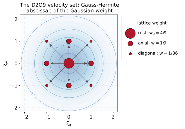
../../_images/gauss_hermite_velocity_set.svg — The D2Q9 velocity set seen as Gauss-Hermite quadrature: its nine velocities \(\boldsymbol{c}_i\) are the abscissae and its weights \(w_i\) are the quadrature weights of the Gaussian equilibrium.¶

D3Q27 vs D3Q19

D3Q27 carries enough abscissae to integrate the complete third-order Hermite expansion exactly, which is why it is the preferred production set for LES. D3Q15 and D3Q19 have fewer abscissae and each needs a small correction to the third-order term, discussed on the collision operators page.

Once the velocities are fixed, the continuous distribution \(f(\boldsymbol{x}, \boldsymbol{\xi}, t)\) collapses to a finite set of populations \(f_i(\boldsymbol{x}, t)\), one per discrete velocity \(\boldsymbol{c}_i\). The moment integrals of the kinetic primer become moment sums, and the BGK relaxation becomes an equation for these populations, derived next.

The discrete equation¶

The discrete version of the Boltzmann equation is the lattice Boltzmann equation, which with the BGK collision operator is written as (Qian et al.[4]):

(2)¶\[ f_i(\boldsymbol{x} + \boldsymbol{c}_i \Delta t, t+\Delta t) - f_i(\boldsymbol{x}, t) = - \omega\bigg[f_i(\boldsymbol{x}, t)-f_i^\mathrm{eq}(\boldsymbol{x}, t)\bigg] + \Delta t\left(1-\frac{\omega}{2}\right)F_i(\boldsymbol{x}, t) \]

where \(f_i\) are the so-called populations and \(\omega = \Delta t / \tau\) is the non-dimensional relaxation frequency. The \(i\) directions are set according to a discrete lattice such as the classical D3Q27. The above equation is also discrete in space and time according to a finite-difference scheme He and Luo[5]. While \(x\) sits on a cartesian grid with spacing \(\Delta x\), \(t\) advances in uniform time-steps \(\Delta t\); in lattice units \(\Delta x = \Delta t = 1\). \(c_s\) is the speed of sound, used extensively as a scaling factor in the LBM context, with \(c_s^2 = 1/3\) in lattice units. It is convenient to introduce the inverse-sound-speed-squared factor \(a_\mathrm{s}^2 = 1/c_s^2 = 3\), which appears throughout the Hermite-based expressions. \(Q_{i\alpha\beta} = c_{i\alpha}c_{i\beta} - c_s^2\delta_{\alpha\beta}\) is the scaled second-order Hermite polynomial and \(\delta_{\alpha\beta}\) is the Kronecker delta. The discrete-velocity force follows Guo et al.[6]:

(3)¶\[ F_i = w_i\left[ a_\mathrm{s}^2 c_{i\alpha} F_\alpha + \frac{1}{2} a_\mathrm{s}^4 \left( F_\alpha u_\beta + F_\beta u_\alpha\right)Q_{i\alpha\beta}\right] \]

The moments from discrete velocity force are:

(4)¶\[ \sum_{i}F_{i}=0 \]

(5)¶\[ \sum_{i}F_{i}c_{i,\alpha}=F_{\alpha} \]

(6)¶\[ \sum_{i}F_{i}c_{i,\alpha}c_{i,\beta}=F_{\alpha}u_{\beta} + F_{\beta}u_{\alpha} \]

Flow Evolution¶

The lattice Boltzmann equation proceeds in two stages, named collision and streaming. The right-hand side of the Eq (2) is solved first at collision, where we make \(f_{i}=f_{i}^{\mathrm{eq}}+f_{i}^{\mathrm{neq}}\):

(7)¶\[ f_i^* = \left(1 - \omega\right)f_{i}^{\mathrm{neq}} + f_i^\mathrm{eq} + \Delta t \left(1 - \frac{\omega}{2}\right) F_i \]

The corresponding amount is called post-collision population, denoted with an asterisk. The final step needed to solve the lattice Boltzmann equation is called streaming, which is a shift of the post-collision populations along their velocity directions:

(8)¶\[ f_{i}(\boldsymbol{x} + \boldsymbol{c}_{i} \Delta t, t+\Delta t) = f_{i}^{*}(\boldsymbol{x}, t) \]

The collision/streaming procedures account for the evolution of the flow.

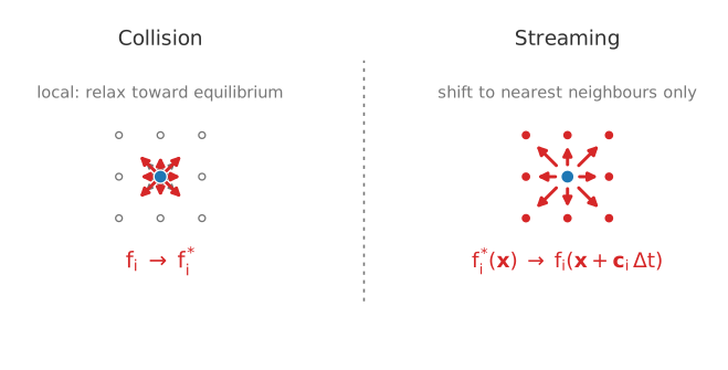
../../_images/collide_stream.svg — The lattice Boltzmann update in two steps. Collision is local: at each node the populations relax toward equilibrium, \(f_i \rightarrow f_i^{*}\), with no neighbour interaction. Streaming then shifts each post-collision population one node along its discrete velocity. The locality of collision and the nearest-neighbour reach of streaming are what make the method map so well onto the GPU.¶

Why this matters for the GPU

This two-step structure, a purely local collision followed by a fixed shift to neighbours, is what makes the method so well suited to GPUs: no node ever needs data from far away. The same locality is why the solver scales to large turbulent domains.

Next steps¶

So far the equilibrium and the collision have been used at their simplest. The next page examines the collision operator in detail, starting from why plain BGK becomes unstable for high-Reynolds LES and how regularization fixes it.