Scaling

Nassu uses a grid refinement by a factor of two \((\Delta x_f = \Delta x_c / 2)\), which gives a general spatial resolution of

(1)\[ \Delta x_n = \frac{\Delta x_0}{2^n} \]

For the temporal scaling, there are two popular options. The diffusive scaling is \(\Delta t \sim \Delta x^2\); it gives a constant relaxation frequency between levels. The acoustic scaling is \(\Delta t \sim \Delta x\); it gives a constant mesoscopic velocity \((\Delta x / \Delta t)\) between levels. Nassu uses the latter:

(2)\[ \Delta t_n = \frac{\Delta t_0}{2^n} \]

This means that each iteration over a coarser level requires two iterations over a finer level. The acoustic scaling keeps the Mach number constant between levels, because the mesoscopic velocity is the same.

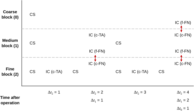
Acoustic scaling on a 2:1 interface: the fine grid advances two steps for every coarse step, exchanging interface data at the shared time levels. Each level collides (CS) on its own step, while the interface communications (IC) only line up where the time levels coincide, so the coarse-to-fine and fine-to-coarse exchanges happen at the common instants.

Acoustic vs diffusive scaling

Diffusive scaling (\(\Delta t \sim \Delta x^2\)) keeps the relaxation frequency constant between levels but advances the fine grid four times per coarse step, which is costly. Acoustic scaling (\(\Delta t \sim \Delta x\)) instead keeps the mesoscopic velocity, and therefore the Mach number, constant between levels, at the price of rescaling the relaxation between levels. Nassu uses the acoustic scaling: a constant Mach number is the natural fit for the weakly-compressible LBM, where Ma must stay small everywhere.

In order to keep the Reynolds number constant, there is a requirement on the lattice-unit viscosity (the physical viscosity is identical across levels; only its lattice-unit value differs):

(3)\[ \nu_{0,f} = 2\nu_{0,c} \]

Similarly, the lattice-unit force density is scaled such that its non-dimensional (physical) value is constant throughout all levels:

(4)\[ F_{\alpha, n} = \frac{\Delta t_n}{\Delta t_0}F_{\alpha, 0} = \frac{F_{\alpha, 0}}{2^n} \]

Notice that this scaling ensures \(F_n/\Delta t_n = F_0/\Delta t_0\). The scaling performed at the interface between levels must assure that the macroscopic moments (\(\rho\), \(\rho u_{\alpha}\) and \(\sigma_{\alpha\beta}\)) remain continuous throughout the simulation domain.

The LBM populations at interface are built through summation of their equilibrium and non-equilibrium populations \(\left(f_{i}=f_{i}^{\mathrm{eq}}+f_{i}^{\mathrm{neq}}\right)\), which can be calculated from the macroscopics \(\left(\rho,u_{\alpha},S_{\alpha\beta}\right)\). The shear stress \(\sigma_{\alpha\beta} = 2\rho\left(\nu_0 + \nu_{SGS}\right)S_{\alpha\beta}\) matched at the interface is carried by the non-equilibrium moment \(\Pi_{\alpha\beta}^{\mathrm{neq}}\) that is actually stored and communicated, since \(S_{\alpha\beta}\) and \(\Pi_{\alpha\beta}^{\mathrm{neq}}\) are linked algebraically (see Macroscopics).

Warning

The shear stress must be matched, not copied

Continuity at an interface is imposed on the moments \(\rho\), \(\rho u_{\alpha}\) and the shear stress \(\sigma_{\alpha\beta}\) (not on the populations directly). Because the relaxation frequency differs between levels, the rate-of-strain \(S_{\alpha\beta}\) that produces a given \(\sigma_{\alpha\beta}\) is different on each side. Reconstructing the populations from a copied \(S_{\alpha\beta}\) instead of the matched \(\sigma_{\alpha\beta}\) makes the stress discontinuous at every refinement boundary and corrupts the LES solution. The rescaling that keeps the stress continuous across levels is derived in the LES SGS scaling section.