Atmospheric Boundary Layer
The simulation of a atmospheric flow is used for the confirmation wether the solver is able to reproduce a wind tunnel experiment. Through appropriate obstacles arrangement, it is possible to shape the wind profile of a wind tunnel in accordance to wind standards for different wind categories. In the present simulations, plate shaped obstacles are placed over a wind tunnel from inlet. To reduce the development length, the Synthetic Eddy Method is adopted as inlet boundary condition:

[1]:
from nassu.cfg.model import ConfigScheme

filename = "tests/validation/cases/06_atmospheric_flow.nassu.yaml"

sim_cfgs = ConfigScheme.sim_cfgs_from_file_dct(filename)
Velocity Profile
Here the functions used for and turbulent intensity velocity profiles processing used for all cases are defined:
[2]:
import pandas as pd
import numpy as np
import matplotlib.pyplot as plt
import pathlib
from nassu.cfg.schemes.simul import SimulationConfigs
from tests.validation.notebooks import common
from vtkmodules.util.numpy_support import vtk_to_numpy

common.use_style()
The floor is delineated with an IBM plane placed at 5.01 nodes height. The scale adopted is such that each LBM node at level 0 correspond to 8 meters. The highest level adopted is 1, with a resolution of 4 meters per node. Only the plates height varied between each case. The plates width was of 12 meters and its spacing of 32x64 meters.
[3]:
base_height = 5.01
max_height_nodes = 25
height_m_node_lvl0 = 8
n_points = 50


def get_line_for_probe(sim_cfg: SimulationConfigs, x_dist: float) -> np.ndarray:
    global base_height, max_height_nodes, n_points
    ds = sim_cfg.domain.domain_size

    p0 = np.array((x_dist, ds.y // 2, base_height))
    p1 = np.array((x_dist, ds.y // 2, base_height + max_height_nodes))
    pos = np.linspace(p0, p1, num=n_points, endpoint=True)

    return pos
[4]:
all_readers_outputs = {}


def get_output(sim_cfg: SimulationConfigs):
    global all_readers_outputs

    key = (sim_cfg.name, sim_cfg.sim_id)
    if key in all_readers_outputs:
        return all_readers_outputs[key]
    else:
        # Avoid keeping too many outputs in memory
        all_readers_outputs = {}

    stats_export = sim_cfg.output.stats["full_stats"]
    last_step = stats_export.interval.get_all_process_steps(sim_cfg.n_steps)[-1]
    data = stats_export.read_export(last_step)

    all_readers_outputs[key] = data
    return all_readers_outputs[key]
[5]:
def get_macr_values(
    sim_cfg: SimulationConfigs, macr_name: str, is_2nd_order: bool, line: np.ndarray
) -> np.ndarray:
    reader_output = get_output(sim_cfg)

    macr_name_read = macr_name if not is_2nd_order else f"{macr_name}_2nd"

    line = common.create_line(line[0], line[-1], len(line) - 1)

    probe_filter = common.probe_over_line(line, reader_output)
    arr = probe_filter.GetOutput().GetPointData().GetArray(macr_name_read)
    probed_data = vtk_to_numpy(arr)

    return probed_data
Load the comparison data generated using the EU standard for wind categories.
[6]:
comparison_folder = pathlib.Path("fixture/SEM/category_vprofile")
files = [
    "profile_log_cat0_H150_Uh0.06",
    "profile_log_cat1_H150_Uh0.06",
    "profile_log_cat2_H150_Uh0.06",
    "profile_log_cat3_H150_Uh0.06",
    "profile_log_cat4_H150_Uh0.06",
]
get_filename_csv = lambda f: comparison_folder / (f + ".csv")


df_eu = {f: pd.read_csv(get_filename_csv(f), delimiter=",") for f in files}

for f in files:
    df_eu[f]["Ix"] = (df_eu[f]["Rxx"] / (df_eu[f]["ux"] ** 2)) ** 0.5
    df_eu[f]["zmeters"] = df_eu[f]["z"]
Power Spectral Density
Here the functions used for the power spectral density (PSD) processing used for all cases are defined:
[7]:
import scipy
from scipy.ndimage import gaussian_filter
[8]:
def filter_avg_data(data):
    data = gaussian_filter(data, sigma=0)
    return data


def theoretical_spectrum_x(f_array):
    S_out = np.zeros(len(f_array))
    for i in range(len(f_array)):
        S_out[i] = 6.8 * f_array[i] / (1 + 10.2 * (f_array[i])) ** (5 / 3)
    return S_out


def numerical_spectrum(data_arr, f, L):
    arr = np.array(data_arr, dtype=np.float32).flatten()

    xf, yf_img = scipy.signal.periodogram(arr, f, scaling="density")
    avg = np.average(arr)
    st = np.std(arr)
    yf_img = yf_img * (xf) / (st * st)
    xf = xf * (L / avg)

    yf = np.real(yf_img)
    return xf, yf
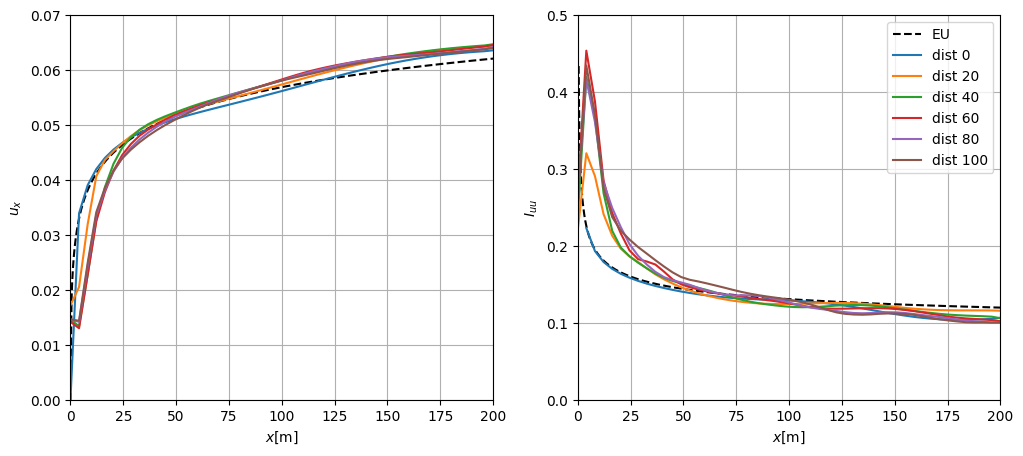
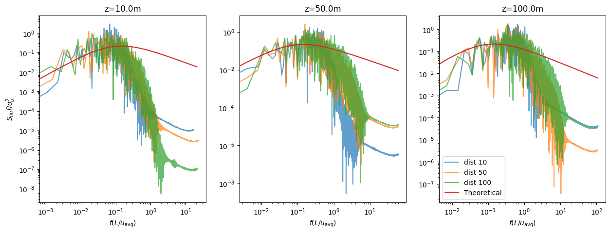
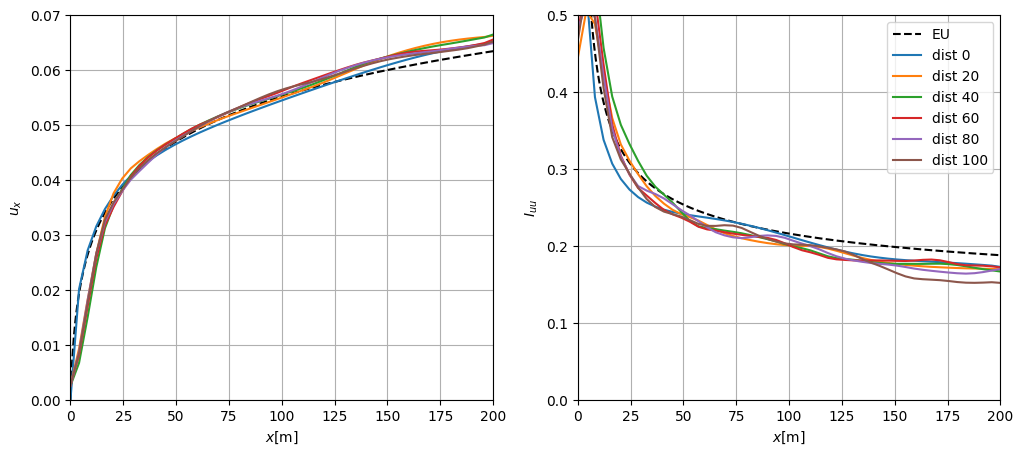
Category 0
For the category 0, no obstacles are placed on the plane.
[9]:
sim_cfg = sim_cfgs["category_0_s4m", 0]

fig, ax = common.fig_double()

ax[0].plot(
    df_eu["profile_log_cat0_H150_Uh0.06"]["zmeters"],
    df_eu["profile_log_cat0_H150_Uh0.06"]["ux"],
    **common.markers.exp_line(linestyle="--"),
    label="EU",
)
ax[1].plot(
    df_eu["profile_log_cat0_H150_Uh0.06"]["zmeters"],
    df_eu["profile_log_cat0_H150_Uh0.06"]["Ix"],
    **common.markers.exp_line(linestyle="--"),
    label="EU",
)

for dist in [0, 20, 40, 60, 80, 100]:
    line01 = get_line_for_probe(sim_cfg, dist)

    ux = get_macr_values(sim_cfg, "ux", is_2nd_order=False, line=line01)
    ux_2nd = get_macr_values(sim_cfg, "ux", is_2nd_order=True, line=line01)
    Ix = ((ux_2nd - (ux**2)) / (ux**2)) ** (0.5)

    normline = ((line01) - base_height) * height_m_node_lvl0

    ax[0].plot(normline[:, 2], ux, label=f"dist {dist}")
    ax[1].plot(normline[:, 2], Ix, label=f"dist {dist}")

ax[0].set_ylabel(r"$u_{x}$")
ax[0].set_xlabel(r"$x$[m]")
ax[0].set_ylim(0, 0.07)
ax[0].set_xlim(0, 200)

ax[1].set_ylabel(r"$I_{uu}$")
ax[1].set_xlabel(r"$x$[m]")
ax[1].legend()
ax[1].set_ylim(0, 0.5)
ax[1].set_xlim(0, 200)

plt.tight_layout()
plt.show(fig)
/tmp/ipykernel_1558238/724278958.py:23: RuntimeWarning: invalid value encountered in divide
  Ix = ((ux_2nd - (ux**2)) / (ux**2)) ** (0.5)
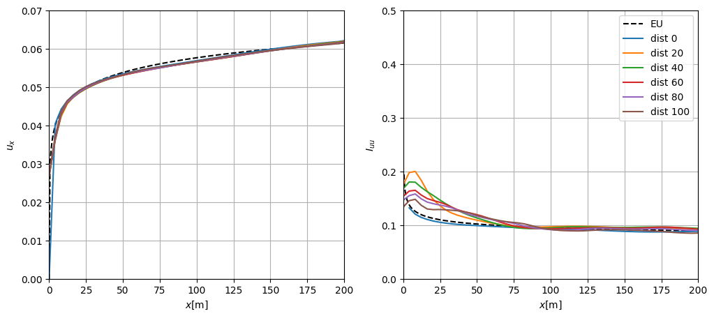
It can be noticed a elevated turbulent intensity at low heigth. It must be highlighted that in the first two nodes after the floor, the IBM has its diffusive layer which may contributes to generate turbulence higher than desired near the ground. Such effect could be mitigated by adopting a higher resolution for a terrain with no obstacles.
[10]:
def read_df_spectrum(sim_cfg: SimulationConfigs, line_name: str):
    spectrum_series = sim_cfg.output.series["velocity"].lines[line_name]

    df_hs = spectrum_series.read_full_data("ux")
    df_points = pd.read_csv(spectrum_series.points_filename)
    df_hs = df_hs[df_hs["time_step"] >= 10000]

    return df_hs, df_points
[11]:
pitot_position_x = [10, 50, 100]
pitot_position_y = [80]
pitot_position_z = [10, 50, 100]
freq = 1

pitot_position_z = [round(z * 0.125 + base_height, 4) for z in pitot_position_z]

df_spectrum = []
df_points = []

for pos in pitot_position_x:
    if pos < 100:
        df_spectrum_aux, df_points_aux = read_df_spectrum(sim_cfg, f"velocity_profile_0{pos}")
    else:
        df_spectrum_aux, df_points_aux = read_df_spectrum(sim_cfg, f"velocity_profile_{pos}")
    df_spectrum.append(df_spectrum_aux)
    df_points.append(df_points_aux)
[12]:
fig, ax = common.fig_triple()
i = 0

for z in pitot_position_z:
    for y in pitot_position_y:
        for j, x in enumerate(pitot_position_x):
            df_probe_id = df_points[j][
                (df_points[j]["x"] == x) & (df_points[j]["y"] == y) & (df_points[j]["z"] == z)
            ].astype(str)
            df_probe_id.reset_index(inplace=True)
            ux_arr = df_spectrum[j][df_probe_id["idx"]]

            # L = get_L(z0[int(abl_category)], (z - floor)*scale)/scale
            H = z - base_height
            nxf, nyf = numerical_spectrum(ux_arr, freq, H)
            yf_theo = theoretical_spectrum_x(nxf)
            yf_avg = filter_avg_data(nyf)
            ax[i].plot(nxf, yf_avg, label=f"dist {x}", alpha=0.5)
    ax[i].plot(nxf, yf_theo, color=common.colors.exp, linestyle="--", label="Theoretical")
    ax[i].set_title(f"z={(z-base_height)*height_m_node_lvl0:.1f}m")
    ax[i].set_xscale("log")
    ax[i].set_yscale("log")
    ax[i].set_xlabel(r"$f(L/u_{\mathrm{avg}})$")
    i += 1

ax[2].legend(loc="lower left")
ax[0].set_ylabel(r"$S_{uu}f/\sigma_{u}^{2}$")

plt.tight_layout()
plt.show(fig)
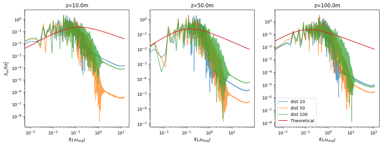
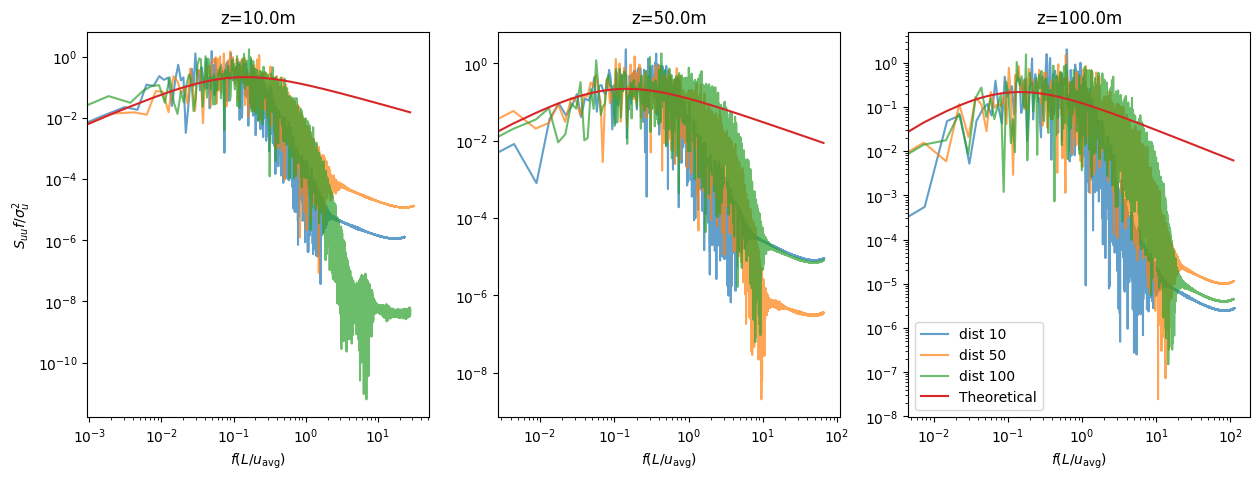
The power spectral density curves suggest that the flow spectra becomes developed around 80 to 90 nodes. Good agreement of the peak with the theoretical Von Karman curve was obtained at all heights measured
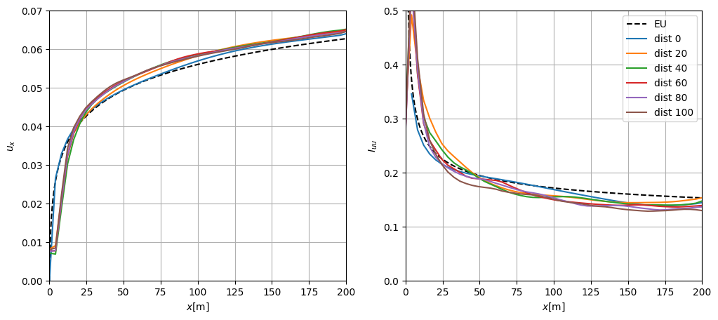
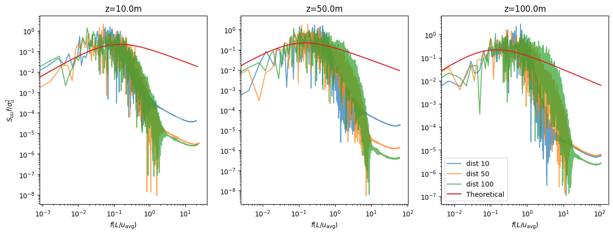
Category I
For the category I, plates of 1 meter heigth were considered.
[13]:
sim_cfg = sim_cfgs["category_1_s4m", 0]

fig, ax = common.fig_double()

ax[0].plot(
    df_eu["profile_log_cat1_H150_Uh0.06"]["zmeters"],
    df_eu["profile_log_cat1_H150_Uh0.06"]["ux"],
    **common.markers.exp_line(linestyle="--"),
    label="EU",
)
ax[1].plot(
    df_eu["profile_log_cat1_H150_Uh0.06"]["zmeters"],
    df_eu["profile_log_cat1_H150_Uh0.06"]["Ix"],
    **common.markers.exp_line(linestyle="--"),
    label="EU",
)

for dist in [0, 20, 40, 60, 80, 100]:
    line01 = get_line_for_probe(sim_cfg, dist)

    ux = get_macr_values(sim_cfg, "ux", is_2nd_order=False, line=line01)
    ux_2nd = get_macr_values(sim_cfg, "ux", is_2nd_order=True, line=line01)
    Ix = ((ux_2nd - (ux**2)) / (ux**2)) ** (0.5)

    normline = ((line01) - base_height) * height_m_node_lvl0

    ax[0].plot(normline[:, 2], ux, label=f"dist {dist}")
    ax[1].plot(normline[:, 2], Ix, label=f"dist {dist}")

ax[0].set_ylabel(r"$u_{x}$")
ax[0].set_xlabel(r"$x$[m]")
ax[0].set_ylim(0, 0.07)
ax[0].set_xlim(0, 200)

ax[1].set_ylabel(r"$I_{uu}$")
ax[1].set_xlabel(r"$x$[m]")
ax[1].legend()
ax[1].set_ylim(0, 0.5)
ax[1].set_xlim(0, 200)

plt.tight_layout()
plt.show(fig)
/tmp/ipykernel_1558238/3427536125.py:23: RuntimeWarning: invalid value encountered in divide
  Ix = ((ux_2nd - (ux**2)) / (ux**2)) ** (0.5)
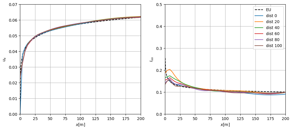
Some improvement of from category 0 results was obtained in this case, however the plates heigth occupies only half node in the most refined level. This might not be ideal to obtain the exact turbulent intensity profile. Nevertheless, the profile fit can be considered as very satisfactory.
[14]:
pitot_position_x = [10, 50, 100]
pitot_position_y = [80]
pitot_position_z = [10, 50, 100]
freq = 1

pitot_position_z = [round(z * 0.125 + base_height, 4) for z in pitot_position_z]

df_spectrum = []
df_points = []

for pos in pitot_position_x:
    if pos < 100:
        df_spectrum_aux, df_points_aux = read_df_spectrum(sim_cfg, f"velocity_profile_0{pos}")
    else:
        df_spectrum_aux, df_points_aux = read_df_spectrum(sim_cfg, f"velocity_profile_{pos}")
    df_spectrum.append(df_spectrum_aux)
    df_points.append(df_points_aux)
[15]:
fig, ax = common.fig_triple()
i = 0

for z in pitot_position_z:
    for y in pitot_position_y:
        for j, x in enumerate(pitot_position_x):
            df_probe_id = df_points[j][
                (df_points[j]["x"] == x) & (df_points[j]["y"] == y) & (df_points[j]["z"] == z)
            ].astype(str)
            df_probe_id.reset_index(inplace=True)
            ux_arr = df_spectrum[j][df_probe_id["idx"]]

            # L = get_L(z0[int(abl_category)], (z - floor)*scale)/scale
            H = z - base_height
            nxf, nyf = numerical_spectrum(ux_arr, freq, H)
            yf_theo = theoretical_spectrum_x(nxf)
            yf_avg = filter_avg_data(nyf)
            ax[i].plot(nxf, yf_avg, label=f"dist {x}", alpha=0.5)
    ax[i].plot(nxf, yf_theo, color=common.colors.exp, linestyle="--", label="Theoretical")
    ax[i].set_title(f"z={(z-base_height)*height_m_node_lvl0:.1f}m")
    ax[i].set_xscale("log")
    ax[i].set_yscale("log")
    ax[i].set_xlabel(r"$f(L/u_{\mathrm{avg}})$")
    i += 1

ax[2].legend(loc="lower left")
ax[0].set_ylabel(r"$S_{uu}f/\sigma_{u}^{2}$")

plt.tight_layout()
plt.show(fig)
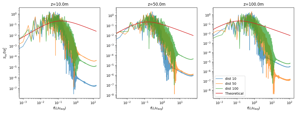
Again, the spectrum seem to become developed between 80 and 90 nodes from inlet.
Category II
To mantain the category II profiles, plates of 2m high were used.
[16]:
sim_cfg = sim_cfgs["category_2_s4m", 0]

fig, ax = common.fig_double()

ax[0].plot(
    df_eu["profile_log_cat2_H150_Uh0.06"]["zmeters"],
    df_eu["profile_log_cat2_H150_Uh0.06"]["ux"],
    **common.markers.exp_line(linestyle="--"),
    label="EU",
)
ax[1].plot(
    df_eu["profile_log_cat2_H150_Uh0.06"]["zmeters"],
    df_eu["profile_log_cat2_H150_Uh0.06"]["Ix"],
    **common.markers.exp_line(linestyle="--"),
    label="EU",
)

for dist in [0, 20, 40, 60, 80, 100]:
    line01 = get_line_for_probe(sim_cfg, dist)

    ux = get_macr_values(sim_cfg, "ux", is_2nd_order=False, line=line01)
    ux_2nd = get_macr_values(sim_cfg, "ux", is_2nd_order=True, line=line01)
    Ix = ((ux_2nd - (ux**2)) / (ux**2)) ** (0.5)

    normline = ((line01) - base_height) * height_m_node_lvl0

    ax[0].plot(normline[:, 2], ux, label=f"dist {dist}")
    ax[1].plot(normline[:, 2], Ix, label=f"dist {dist}")

ax[0].set_ylabel(r"$u_{x}$")
ax[0].set_xlabel(r"$x$[m]")
ax[0].set_ylim(0, 0.07)
ax[0].set_xlim(0, 200)

ax[1].set_ylabel(r"$I_{uu}$")
ax[1].set_xlabel(r"$x$[m]")
ax[1].legend()
ax[1].set_ylim(0, 0.5)
ax[1].set_xlim(0, 200)

plt.tight_layout()
plt.show(fig)
/tmp/ipykernel_1558238/1378197960.py:23: RuntimeWarning: invalid value encountered in divide
  Ix = ((ux_2nd - (ux**2)) / (ux**2)) ** (0.5)
It can be seen good agreement from around 15m and above. To improve the results below this height a finer grid to correctly compute the elevated velocity gradient would be necessary.
[17]:
pitot_position_x = [10, 50, 100]
pitot_position_y = [80]
pitot_position_z = [10, 50, 100]
freq = 1

pitot_position_z = [round(z * 0.125 + base_height, 4) for z in pitot_position_z]

df_spectrum = []
df_points = []

for pos in pitot_position_x:
    if pos < 100:
        df_spectrum_aux, df_points_aux = read_df_spectrum(sim_cfg, f"velocity_profile_0{pos}")
    else:
        df_spectrum_aux, df_points_aux = read_df_spectrum(sim_cfg, f"velocity_profile_{pos}")
    df_spectrum.append(df_spectrum_aux)
    df_points.append(df_points_aux)
[18]:
fig, ax = common.fig_triple()
i = 0

for z in pitot_position_z:
    for y in pitot_position_y:
        for j, x in enumerate(pitot_position_x):
            df_probe_id = df_points[j][
                (df_points[j]["x"] == x) & (df_points[j]["y"] == y) & (df_points[j]["z"] == z)
            ].astype(str)
            df_probe_id.reset_index(inplace=True)
            ux_arr = df_spectrum[j][df_probe_id["idx"]]

            # L = get_L(z0[int(abl_category)], (z - floor)*scale)/scale
            H = z - base_height
            nxf, nyf = numerical_spectrum(ux_arr, freq, H)
            yf_theo = theoretical_spectrum_x(nxf)
            yf_avg = filter_avg_data(nyf)
            ax[i].plot(nxf, yf_avg, label=f"dist {x}", alpha=0.5)
    ax[i].plot(nxf, yf_theo, color=common.colors.exp, linestyle="--", label="Theoretical")
    ax[i].set_title(f"z={(z-base_height)*height_m_node_lvl0:.1f}m")
    ax[i].set_xscale("log")
    ax[i].set_yscale("log")
    ax[i].set_xlabel(r"$f(L/u_{\mathrm{avg}})$")
    i += 1

ax[2].legend(loc="lower left")
ax[0].set_ylabel(r"$S_{uu}f/\sigma_{u}^{2}$")

plt.tight_layout()
plt.show(fig)
The spectrum deviates from theoretical peak at 10 meters possibly due to influence of obstacles, a simulation at higher resolution could also change this aspect. Above this height the spectrum tends to follow the theoretical Von Karman curve.
Category III
To mantain the category III profile from inlet, plates of 6 meters were adopted.
[19]:
sim_cfg = sim_cfgs["category_3_s4m", 0]

fig, ax = common.fig_double()

ax[0].plot(
    df_eu["profile_log_cat3_H150_Uh0.06"]["zmeters"],
    df_eu["profile_log_cat3_H150_Uh0.06"]["ux"],
    **common.markers.exp_line(linestyle="--"),
    label="EU",
)
ax[1].plot(
    df_eu["profile_log_cat3_H150_Uh0.06"]["zmeters"],
    df_eu["profile_log_cat3_H150_Uh0.06"]["Ix"],
    **common.markers.exp_line(linestyle="--"),
    label="EU",
)

for dist in [0, 20, 40, 60, 80, 100]:
    line01 = get_line_for_probe(sim_cfg, dist)

    ux = get_macr_values(sim_cfg, "ux", is_2nd_order=False, line=line01)
    ux_2nd = get_macr_values(sim_cfg, "ux", is_2nd_order=True, line=line01)
    Ix = ((ux_2nd - (ux**2)) / (ux**2)) ** (0.5)

    normline = ((line01) - base_height) * height_m_node_lvl0

    ax[0].plot(normline[:, 2], ux, label=f"dist {dist}")
    ax[1].plot(normline[:, 2], Ix, label=f"dist {dist}")

ax[0].set_ylabel(r"$u_{x}$")
ax[0].set_xlabel(r"$x$[m]")
ax[0].set_ylim(0, 0.07)
ax[0].set_xlim(0, 200)

ax[1].set_ylabel(r"$I_{uu}$")
ax[1].set_xlabel(r"$x$[m]")
ax[1].legend()
ax[1].set_ylim(0, 0.5)
ax[1].set_xlim(0, 200)

plt.tight_layout()
plt.show(fig)
/tmp/ipykernel_1558238/2752850397.py:23: RuntimeWarning: invalid value encountered in divide
  Ix = ((ux_2nd - (ux**2)) / (ux**2)) ** (0.5)
In this case, the turbulence occurs in larger scales and the obstacles are better perceived by the simulation since they occupy more than a single node.The obtained profiles over the domain have excellent agreement with the inlet profile.
[20]:
pitot_position_x = [10, 50, 100]
pitot_position_y = [80]
pitot_position_z = [10, 50, 100]
freq = 1

pitot_position_z = [round(z * 0.125 + base_height, 4) for z in pitot_position_z]

df_spectrum = []
df_points = []

for pos in pitot_position_x:
    if pos < 100:
        df_spectrum_aux, df_points_aux = read_df_spectrum(sim_cfg, f"velocity_profile_0{pos}")
    else:
        df_spectrum_aux, df_points_aux = read_df_spectrum(sim_cfg, f"velocity_profile_{pos}")
    df_spectrum.append(df_spectrum_aux)
    df_points.append(df_points_aux)
[21]:
fig, ax = common.fig_triple()
i = 0

for z in pitot_position_z:
    for y in pitot_position_y:
        for j, x in enumerate(pitot_position_x):
            df_probe_id = df_points[j][
                (df_points[j]["x"] == x) & (df_points[j]["y"] == y) & (df_points[j]["z"] == z)
            ].astype(str)
            df_probe_id.reset_index(inplace=True)
            ux_arr = df_spectrum[j][df_probe_id["idx"]]

            # L = get_L(z0[int(abl_category)], (z - floor)*scale)/scale
            H = z - base_height
            nxf, nyf = numerical_spectrum(ux_arr, freq, H)
            yf_theo = theoretical_spectrum_x(nxf)
            yf_avg = filter_avg_data(nyf)
            ax[i].plot(nxf, yf_avg, label=f"dist {x}", alpha=0.5)
    ax[i].plot(nxf, yf_theo, color=common.colors.exp, linestyle="--", label="Theoretical")
    ax[i].set_title(f"z={(z-base_height)*height_m_node_lvl0:.1f}m")
    ax[i].set_xscale("log")
    ax[i].set_yscale("log")
    ax[i].set_xlabel(r"$f(L/u_{\mathrm{avg}})$")
    i += 1

ax[2].legend(loc="lower left")
ax[0].set_ylabel(r"$S_{uu}f/\sigma_{u}^{2}$")

plt.tight_layout()
plt.show(fig)
Again, the curve at 10 meters seems to be displaced. In general, the spectrum seems to develop earlier in comparison to the previous categories.
Category IV
The plates used to maintain the category IV profile were 10 meters high.
[22]:
sim_cfg = sim_cfgs["category_4_s4m", 0]

fig, ax = common.fig_double()

ax[0].plot(
    df_eu["profile_log_cat4_H150_Uh0.06"]["zmeters"],
    df_eu["profile_log_cat4_H150_Uh0.06"]["ux"],
    **common.markers.exp_line(linestyle="--"),
    label="EU",
)
ax[1].plot(
    df_eu["profile_log_cat4_H150_Uh0.06"]["zmeters"],
    df_eu["profile_log_cat4_H150_Uh0.06"]["Ix"],
    **common.markers.exp_line(linestyle="--"),
    label="EU",
)

for dist in [0, 20, 40, 60, 80, 100]:
    line01 = get_line_for_probe(sim_cfg, dist)

    ux = get_macr_values(sim_cfg, "ux", is_2nd_order=False, line=line01)
    ux_2nd = get_macr_values(sim_cfg, "ux", is_2nd_order=True, line=line01)
    Ix = ((ux_2nd - (ux**2)) / (ux**2)) ** (0.5)

    normline = ((line01) - base_height) * height_m_node_lvl0

    ax[0].plot(normline[:, 2], ux, label=f"dist {dist}")
    ax[1].plot(normline[:, 2], Ix, label=f"dist {dist}")

ax[0].set_ylabel(r"$u_{x}$")
ax[0].set_xlabel(r"$x$[m]")
ax[0].set_ylim(0, 0.07)
ax[0].set_xlim(0, 200)

ax[1].set_ylabel(r"$I_{uu}$")
ax[1].set_xlabel(r"$x$[m]")
ax[1].legend()
ax[1].set_ylim(0, 0.5)
ax[1].set_xlim(0, 200)

plt.tight_layout()
plt.show(fig)
/tmp/ipykernel_1558238/1666365321.py:23: RuntimeWarning: invalid value encountered in divide
  Ix = ((ux_2nd - (ux**2)) / (ux**2)) ** (0.5)
Excellent agreement between the developed profile and the EU standard for the category IV was obtained.
[23]:
pitot_position_x = [10, 50, 100]
pitot_position_y = [80]
pitot_position_z = [10, 50, 100]
freq = 1

pitot_position_z = [round(z * 0.125 + base_height, 4) for z in pitot_position_z]

df_spectrum = []
df_points = []

for pos in pitot_position_x:
    if pos < 100:
        df_spectrum_aux, df_points_aux = read_df_spectrum(sim_cfg, f"velocity_profile_0{pos}")
    else:
        df_spectrum_aux, df_points_aux = read_df_spectrum(sim_cfg, f"velocity_profile_{pos}")
    df_spectrum.append(df_spectrum_aux)
    df_points.append(df_points_aux)
[24]:
fig, ax = common.fig_triple()
i = 0

for z in pitot_position_z:
    for y in pitot_position_y:
        for j, x in enumerate(pitot_position_x):
            df_probe_id = df_points[j][
                (df_points[j]["x"] == x) & (df_points[j]["y"] == y) & (df_points[j]["z"] == z)
            ].astype(str)
            df_probe_id.reset_index(inplace=True)
            ux_arr = df_spectrum[j][df_probe_id["idx"]]

            # L = get_L(z0[int(abl_category)], (z - floor)*scale)/scale
            H = z - base_height
            nxf, nyf = numerical_spectrum(ux_arr, freq, H)
            yf_theo = theoretical_spectrum_x(nxf)
            yf_avg = filter_avg_data(nyf)
            ax[i].plot(nxf, yf_avg, label=f"dist {x}", alpha=0.5)
    ax[i].plot(nxf, yf_theo, color=common.colors.exp, linestyle="--", label="Theoretical")
    ax[i].set_title(f"z={(z-base_height)*height_m_node_lvl0:.1f}m")
    ax[i].set_xscale("log")
    ax[i].set_yscale("log")
    ax[i].set_xlabel(r"$f(L/u_{\mathrm{avg}})$")
    i += 1

ax[2].legend(loc="lower left")
ax[0].set_ylabel(r"$S_{uu}f/\sigma_{u}^{2}$")

plt.tight_layout()
plt.show(fig)
In this case the spectrum seems to develop even earlier in comparison to previous simulations.
Version
[25]:
sim_info = sim_cfg.output.read_info()

nassu_commit = sim_info["commit"]
nassu_version = sim_info["version"]
print("Version:", nassu_version)
print("Commit hash:", nassu_commit)
Version: 1.6.45
Commit hash: a2287d74877f61304fc618ad5e2c77a25b3f7f39
Configuration
[26]:
from IPython.display import Code

Code(filename=filename)
[26]:
variables:
simul:
dev_time: 10000
stats_time: 60000
scale: !math 1/8
plane_height: 5.01
sigma_sem: 20
domain:
length: 600
width: 160
height: 112
refine: &ANCHOR_VOLUMES_REFINE
- start: [0.0, 55.0, 0.0]
end: [336.0, 105.0, 32.0]
lvl: 1
is_abs: true
var:
15m_height: !math ${simul.plane_height} + (15 * ${simul.scale})
150m_height: !math ${simul.plane_height} + (150 * ${simul.scale})
## Same variables to dependencies
simulations:
- name: category_0_s4m
save_path: ./tests/validation/results/06_atmospheric_flow
run_simul: true
n_steps: !math "${simul.dev_time} + ${simul.stats_time}"
report:
frequency: 500
checkpoint:
export:
interval: { frequency: 10000, start_step: !math "${simul.dev_time}" }
finish_save: true
keep_only_last_checkpoint: true
data:
divergence: { frequency: 1 }
monitors:
fields:
macrs_stats:
macrs: [rho, u]
stats: [min, max, mean]
interval: { start_step: 0, frequency: 10 }
instantaneous:
full_domain: { interval: { frequency: 0 }, macrs: [rho, u] }
statistics:
interval: { frequency: 10, start_step: !sub "${simul.dev_time}" }
macrs_1st_order: [rho, u]
macrs_2nd_order: [u]
exports:
full_stats: { interval: { frequency: 0 } }
probes:
historic_series:
velocity:
macrs: ["u"]
interval: { frequency: 2, lvl: 0, start_step: !sub "${simul.dev_time}" }
lines:
velocity_profile_000:
dist: 0.0625
start_pos: !math [0, "0.5*${domain.width}", "${simul.plane_height}"]
end_pos: !math [0, "0.5*${domain.width}", "${simul.plane_height} + 64"]
velocity_profile_010:
dist: 0.0625
start_pos: !math [10, "0.5*${domain.width}", "${simul.plane_height}"]
end_pos: !math [10, "0.5*${domain.width}", "${simul.plane_height} + 64"]
velocity_profile_020:
dist: 0.0625
start_pos: !math [20, "0.5*${domain.width}", "${simul.plane_height}"]
end_pos: !math [20, "0.5*${domain.width}", "${simul.plane_height} + 64"]
velocity_profile_030:
dist: 0.0625
start_pos: !math [30, "0.5*${domain.width}", "${simul.plane_height}"]
end_pos: !math [30, "0.5*${domain.width}", "${simul.plane_height} + 64"]
velocity_profile_040:
dist: 0.0625
start_pos: !math [40, "0.5*${domain.width}", "${simul.plane_height}"]
end_pos: !math [40, "0.5*${domain.width}", "${simul.plane_height} + 64"]
velocity_profile_050:
dist: 0.0625
start_pos: !math [50, "0.5*${domain.width}", "${simul.plane_height}"]
end_pos: !math [50, "0.5*${domain.width}", "${simul.plane_height} + 64"]
velocity_profile_060:
dist: 0.0625
start_pos: !math [60, "0.5*${domain.width}", "${simul.plane_height}"]
end_pos: !math [60, "0.5*${domain.width}", "${simul.plane_height} + 64"]
velocity_profile_070:
dist: 0.0625
start_pos: !math [70, "0.5*${domain.width}", "${simul.plane_height}"]
end_pos: !math [70, "0.5*${domain.width}", "${simul.plane_height} + 64"]
velocity_profile_080:
dist: 0.0625
start_pos: !math [80, "0.5*${domain.width}", "${simul.plane_height}"]
end_pos: !math [80, "0.5*${domain.width}", "${simul.plane_height} + 64"]
velocity_profile_090:
dist: 0.0625
start_pos: !math [90, "0.5*${domain.width}", "${simul.plane_height}"]
end_pos: !math [90, "0.5*${domain.width}", "${simul.plane_height} + 64"]
velocity_profile_100:
dist: 0.0625
start_pos: !math [100, "0.5*${domain.width}", "${simul.plane_height}"]
end_pos:
!math [100, "0.5*${domain.width}", "${simul.plane_height} + 64"]
velocity_profile_110:
dist: 0.0625
start_pos: !math [110, "0.5*${domain.width}", "${simul.plane_height}"]
end_pos:
!math [110, "0.5*${domain.width}", "${simul.plane_height} + 64"]
velocity_profile_120:
dist: 0.0625
start_pos: !math [120, "0.5*${domain.width}", "${simul.plane_height}"]
end_pos:
!math [120, "0.5*${domain.width}", "${simul.plane_height} + 64"]
velocity_profile_130:
dist: 0.0625
start_pos: !math [130, "0.5*${domain.width}", "${simul.plane_height}"]
end_pos:
!math [130, "0.5*${domain.width}", "${simul.plane_height} + 64"]
velocity_profile_140:
dist: 0.0625
start_pos: !math [140, "0.5*${domain.width}", "${simul.plane_height}"]
end_pos:
!math [140, "0.5*${domain.width}", "${simul.plane_height} + 64"]
velocity_profile_150:
dist: 0.0625
start_pos: !math [150, "0.5*${domain.width}", "${simul.plane_height}"]
end_pos:
!math [150, "0.5*${domain.width}", "${simul.plane_height} + 64"]
velocity_profile_160:
dist: 0.0625
start_pos: !math [160, "0.5*${domain.width}", "${simul.plane_height}"]
end_pos:
!math [160, "0.5*${domain.width}", "${simul.plane_height} + 64"]
velocity_profile_170:
dist: 0.0625
start_pos: !math [170, "0.5*${domain.width}", "${simul.plane_height}"]
end_pos:
!math [170, "0.5*${domain.width}", "${simul.plane_height} + 64"]
velocity_profile_180:
dist: 0.0625
start_pos: !math [180, "0.5*${domain.width}", "${simul.plane_height}"]
end_pos:
!math [180, "0.5*${domain.width}", "${simul.plane_height} + 64"]
velocity_profile_190:
dist: 0.0625
start_pos: !math [190, "0.5*${domain.width}", "${simul.plane_height}"]
end_pos:
!math [190, "0.5*${domain.width}", "${simul.plane_height} + 64"]
velocity_profile_200:
dist: 0.0625
start_pos: !math [200, "0.5*${domain.width}", "${simul.plane_height}"]
end_pos:
!math [200, "0.5*${domain.width}", "${simul.plane_height} + 64"]
velocity_profile_210:
dist: 0.0625
start_pos: !math [210, "0.5*${domain.width}", "${simul.plane_height}"]
end_pos:
!math [210, "0.5*${domain.width}", "${simul.plane_height} + 64"]
long_profile_15m:
dist: 0.125
start_pos:
!math [
0,
"0.5*${domain.width}",
"${simul.plane_height} + ${var.15m_height}",
]
end_pos:
!math [
300,
"0.5*${domain.width}",
"${simul.plane_height} + ${var.15m_height}",
]
long_profile_150m:
dist: 0.125
start_pos:
!math [
0,
"0.5*${domain.width}",
"${simul.plane_height} + ${var.150m_height}",
]
end_pos:
!math [
300,
"0.5*${domain.width}",
"${simul.plane_height} + ${var.150m_height}",
]
domain:
domain_size:
x: !sub "${domain.length}"
y: !sub "${domain.width}"
z: !math "${domain.height}"
block_size: 8
bodies:
full_plane:
IBM:
order: 0
cfg_use: plane_cfg
lnas_path: fixture/lnas/wind_tunnel/full_plane.lnas
small_triangles: add
global_transformations:
- transformation:
translation: !math [0, 0, "${simul.plane_height}"]
point_clouds_apply: []
bodies_apply: ["full_plane"]
probes_apply: []
refinement:
static:
lvl1:
volumes_refine: *ANCHOR_VOLUMES_REFINE
models:
precision:
default: single
LBM:
tau: 0.50001
F:
x: 0
y: 0
z: 0
vel_set: D3Q27
coll_oper: RRBGK
initialization:
sem_field: true
engine:
name: CUDA
BC:
periodic_dims: [false, false, false]
BC_map:
- pos: E
BC: RegularizedNeumannOutlet
rho: 1.0
wall_normal: E
order: 2
- pos: F
BC: Neumann
wall_normal: F
order: 1
- pos: B
BC: RegularizedHWBB
wall_normal: B
order: 1
- pos: N
BC: Neumann
wall_normal: N
order: 0
- pos: S
BC: Neumann
wall_normal: S
order: 0
SEM:
eddies:
lengthscale:
{
x: !sub "${simul.sigma_sem}",
y: !sub "${simul.sigma_sem}",
z: !sub "${simul.sigma_sem}",
}
eddies_vol_density: 300
domain_limits_yz:
start: !math ["${simul.sigma_sem}", "-${simul.sigma_sem}"]
end:
!math [
"${domain.width}-${simul.sigma_sem}",
"${domain.height}-${simul.sigma_sem}",
]
profile:
csv_profile_data: "./fixture/SEM/category_vprofile/profile_log_cat0_H150_Uh0.06.csv"
z_offset: !math "${simul.plane_height}"
length_mul: !math "${simul.scale}"
LES:
model: Smagorinsky
sgs_cte: 0.17
IBM:
dirac_delta: 3_points
forces_accomodate_time: 500
body_cfgs:
default:
n_iterations: 3
forces_factor: 1.0
plane_cfg:
n_iterations: 3
forces_factor: 0.5
kinetic_energy_correction: false
wall_model:
name: EqLog
dist_ref: 3.125
dist_shell: 0.125
start_step: 5000
params:
z0: !math "0.003*${simul.scale}"
TDMA_max_error: 1e-04
TDMA_max_iters: 10
TDMA_min_div: 25
TDMA_max_div: 25
multiblock:
overlap_F2C: 2
- name: category_1_s4m
parent: category_0_s4m
run_simul: true
domain:
bodies:
plates_obstacles:
IBM:
order: 1
lnas_path: fixture/lnas/wind_tunnel/category_I/plates_Nx160Ny70_6x1_spacing16x32_offset19y.lnas
volumes_limits:
body_transformed:
- start: !math [10, 20, 0]
end: !math [300, "${domain.width} - 20", "0.5*${domain.height}"]
small_triangles: add
transformation:
translation: [0, 1, 0]
scale: !math [
"64.0*${simul.scale}",
"64.0*${simul.scale}",
"32.0*${simul.scale}",
] #1m
global_transformations:
- transformation: !not-inherit
translation: !math [0, 0, "${simul.plane_height}"]
point_clouds_apply: []
bodies_apply: ["full_plane", "plates_obstacles"]
probes_apply: []
models:
IBM:
body_cfgs:
plane_cfg:
wall_model:
params:
z0: !math "0.01*${simul.scale}"
BC:
SEM:
profile:
csv_profile_data: "./fixture/SEM/category_vprofile/profile_log_cat1_H150_Uh0.06.csv"
- name: category_2_s4m
parent: category_0_s4m
run_simul: true
domain:
bodies:
plates_obstacles:
IBM:
order: 1
lnas_path: fixture/lnas/wind_tunnel/category_II/plates_Nx160Ny70_6x2_spacing16x32_offset19y.lnas
volumes_limits:
body_transformed:
- start: !math [10, 20, 0]
end: !math [300, "${domain.width} - 20", "${domain.height}"]
small_triangles: add
transformation:
translation: [0, 1, 0]
scale: !math [
"64.0*${simul.scale}",
"64.0*${simul.scale}",
"32.0*${simul.scale}",
] #2m
global_transformations:
- transformation: !not-inherit
translation: !math [0, 0, "${simul.plane_height}"]
point_clouds_apply: []
bodies_apply: ["full_plane", "plates_obstacles"]
probes_apply: []
models:
IBM:
body_cfgs:
plane_cfg:
wall_model:
params:
z0: !math "0.05*${simul.scale}"
BC:
SEM:
profile:
csv_profile_data: "./fixture/SEM/category_vprofile/profile_log_cat2_H150_Uh0.06.csv"
- name: category_3_s4m
parent: category_0_s4m
run_simul: true
domain:
bodies:
plates_obstacles:
IBM:
order: 1
lnas_path: fixture/lnas/wind_tunnel/category_II/plates_Nx160Ny70_6x2_spacing16x32_offset19y.lnas
volumes_limits:
body_transformed:
- start: !math [10, 20, 0]
end: !math [300, "${domain.width} - 20", "${domain.height}"]
small_triangles: add
transformation:
translation: [0, 1, 0]
scale: !math [
"64.0*${simul.scale}",
"64.0*${simul.scale}",
"3*32.0*${simul.scale}",
] #6m
global_transformations:
- transformation: !not-inherit
translation: !math [0, 0, "${simul.plane_height}"]
point_clouds_apply: []
bodies_apply: ["full_plane", "plates_obstacles"]
probes_apply: []
models:
IBM:
body_cfgs:
plane_cfg:
wall_model:
params:
z0: !math "0.3*${simul.scale}"
BC:
SEM:
profile:
csv_profile_data: "./fixture/SEM/category_vprofile/profile_log_cat3_H150_Uh0.06.csv"
- name: category_4_s4m
parent: category_0_s4m
run_simul: true
domain:
bodies:
plates_obstacles:
IBM:
order: 1
lnas_path: fixture/lnas/wind_tunnel/category_II/plates_Nx160Ny70_6x2_spacing16x32_offset19y.lnas
volumes_limits:
body_transformed:
- start: !math [10, 20, 0]
end: !math [300, "${domain.width} - 20", "${domain.height}"]
small_triangles: add
transformation:
translation: [0, 1, 0]
scale: !math [
"64.0*${simul.scale}",
"64.0*${simul.scale}",
"5.0*32.0*${simul.scale}",
] # 10m
global_transformations:
- transformation: !not-inherit
translation: !math [0, 0, "${simul.plane_height}"]
point_clouds_apply: []
bodies_apply: ["full_plane", "plates_obstacles"]
probes_apply: []
models:
IBM:
body_cfgs:
plane_cfg:
wall_model:
params:
z0: !math "1.0*${simul.scale}"
BC:
SEM:
profile:
csv_profile_data: "./fixture/SEM/category_vprofile/profile_log_cat4_H150_Uh0.06.csv"