
 AeroSim Docs
Subgrid models
The filtered equations left us with one unknown: the subgrid viscosity \(\nu_{\mathrm{SGS}}\) that stands in for all the unresolved turbulence. A subgrid model is a recipe for computing that field from the resolved flow. This page motivates the form such a recipe must take, building it from physical reasoning before any specific model is named, so that the Smagorinsky model on the next page appears as the simplest answer to a question rather than a formula to memorise.
Why an eddy viscosity at all
The eddy-viscosity hypothesis of Equation (6) borrows an idea from molecular kinetic theory. In a gas, molecular viscosity arises because random molecular motion transports momentum across a velocity gradient, smoothing it out. Boussinesq’s analogy is to treat the unresolved turbulent eddies the same way: the small eddies churn fluid across the resolved velocity gradients and so transport resolved momentum, an effect that looks, on average, like an enhanced viscosity [1][2]. The analogy is not exact, since turbulent eddies are not small, fast and uncorrelated the way molecules are, but it captures the dominant behaviour the subgrid scales must reproduce: they drain energy from the resolved field and align that drain with the resolved strain rate. For the mostly-dissipative role the subgrid stress plays, this is enough, and it reduces the entire closure problem to estimating a single scalar, \(\nu_{\mathrm{SGS}}\).
The dimensional argument
What can \(\nu_{\mathrm{SGS}}\) possibly depend on? It is a property of the subgrid eddies, so it can only be built from quantities that characterise those eddies. A viscosity has dimensions of length-squared per time, which is the same as a length times a velocity. The cleanest way to construct it is therefore as the product of a characteristic length and a characteristic velocity of the subgrid motion [2][1]:
This is the same scaling that molecular viscosity obeys (mean free path times thermal speed) and that the mixing-length idea uses in RANS. The work of building a model reduces to two choices: which length, and which velocity.
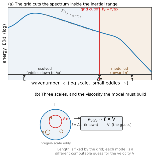
The dimensional argument for the subgrid viscosity. The grid cuts the energy spectrum inside the inertial range; eddies larger than the cutoff (down to \(\Delta x\)) are resolved, smaller ones (toward the Kolmogorov scale \(\eta\)) are modelled. Since \(\nu_{\mathrm{SGS}}\) scales as length times velocity and the length is the grid spacing, every subgrid model is a different computable guess for the velocity of the unresolved eddies.
Key idea
Dimensional analysis collapses the entire closure problem to two choices: a subgrid length and a subgrid velocity. The length is forced by implicit filtering to be the grid spacing \(\Delta x\). Only the velocity scale is left open, so every subgrid model is, at bottom, just a different computable guess for the velocity of the unresolved eddies.
The characteristic length is the only length the subgrid scales know about, namely the filter width, which separates resolved from unresolved motion. With implicit filtering this is the grid spacing, so \(\ell = \Delta x\). Eddies of this size are the largest of the unresolved ones and dominate the subgrid stress; smaller eddies carry progressively less energy and momentum.
The characteristic velocity is the velocity scale of those same eddies. A natural candidate is \(\sqrt{k_{\ell}}\), where \(k_{\ell}\) is the kinetic energy of eddies of size \(\ell\). The problem is that \(k_{\ell}\) is itself a subgrid quantity, unavailable in the simulation, so every subgrid model is essentially a different, computable estimate of this velocity scale in terms of the resolved field. The choice of that estimate is what distinguishes one model from another.
This is exactly where the Smagorinsky model enters: it makes the simplest possible choice for the subgrid velocity scale, tying it directly to the resolved strain rate. That choice, its single calibration constant, and the form it takes inside the lattice Boltzmann solver are developed next.
Limits of validity
No subgrid model is universally best. Which one to use, and the value of its constant, ultimately depends on validation against reference data for the class of flow at hand.