Laminar Flat-Plate Boundary Layer (Blasius)¶

This notebook validates the local skin-friction coefficient Cf(x) of a zero-pressure-gradient laminar boundary layer over a flat plate against the closed-form Blasius similarity solution. The plate is an immersed-boundary (IBM) body, and the wall friction is read from the lean data.body_nodes friction export (issue #879): per source triangle the solver writes the aggregated viscous traction t = 2 rho nu (S . n), and nassu.viz.friction splits it into a wall-normal (pressure) and a wall-tangential (skin-friction) part. For a flat plate the wall is everywhere tangent to the flow, so the traction is essentially pure wall-shear stress and Cf(x) follows directly.

Results require a GPU run. This notebook is committed UNEXECUTED. Run the case on a GPU first:

uv run nassu run validation/external_aero/03_flat_plate_boundary_layer/03_flat_plate_boundary_layer.nassu.yaml

then run all cells; every figure regenerates from the parsed config and the results/ export.

Configuration and parameters¶

The notebook reads every parameter from the parsed YAML, so it always matches the file the solver ran. Nothing is hard-coded.

[ ]:

from nassu.cfg.model import ConfigScheme

filename = (
    "validation/external_aero/03_flat_plate_boundary_layer/03_flat_plate_boundary_layer.nassu.yaml"
)

sim_cfgs = ConfigScheme.sim_cfgs_from_file_dct(filename)
sim_cfg = next(iter(sim_cfgs.values()))
sim_cfg.name

[ ]:

import numpy as np

# Freestream speed from the inlet BC and viscosity from the LBM model (lattice units).
u_inf = max(bc.ux for bc in sim_cfg.models.BC.BC_map if "ux" in bc.model_dump())
nu = sim_cfg.models.LBM.kinematic_viscosity
rho_inf = 1.0

# Plate geometry, taken from the exact placed body so x_le / L match the run.
plate = sim_cfg.domain.bodies["plate"]
verts = np.asarray(plate.lagrangian_fmt.geometry.vertices)
x_le = float(verts[:, 0].min())  # leading-edge x (domain coordinate)
x_te = float(verts[:, 0].max())  # trailing-edge x
plate_length = x_te - x_le

Re_L = u_inf * plate_length / nu
print(f"U_inf = {u_inf}  nu = {nu:.5g}  Ma = {np.sqrt(3) * u_inf:.4f}")
print(f"plate: x_le = {x_le}  x_te = {x_te}  L = {plate_length}")
print(f"Re_L  = {Re_L:.0f}  (laminar; transition ~ 5e5)")

Blasius reference solution¶

For a zero-pressure-gradient laminar boundary layer the local skin-friction coefficient is

{math} C_f(x) = \frac{0.664}{\sqrt{\mathrm{Re}_x}}, \qquad \mathrm{Re}_x = \frac{U_\infty\, x}{\nu},

and the plate-length-averaged value is Cf_bar(Re_L) = 1.328 / sqrt(Re_L). These are the exact similarity constants (Schlichting & Gersten, Boundary-Layer Theory). The committed reference/blasius_cf.csv tabulates the same curve as a provenance record; here we evaluate the formula directly.

[ ]:

def blasius_cf(Re_x):
    """Blasius local skin-friction coefficient."""
    return 0.664 / np.sqrt(Re_x)


def blasius_cf_bar(Re_L):
    """Blasius plate-averaged skin-friction coefficient."""
    return 1.328 / np.sqrt(Re_L)


print("Cf_bar(Re_L) =", blasius_cf_bar(Re_L))

Read the friction export and compute `Cf(x)`¶

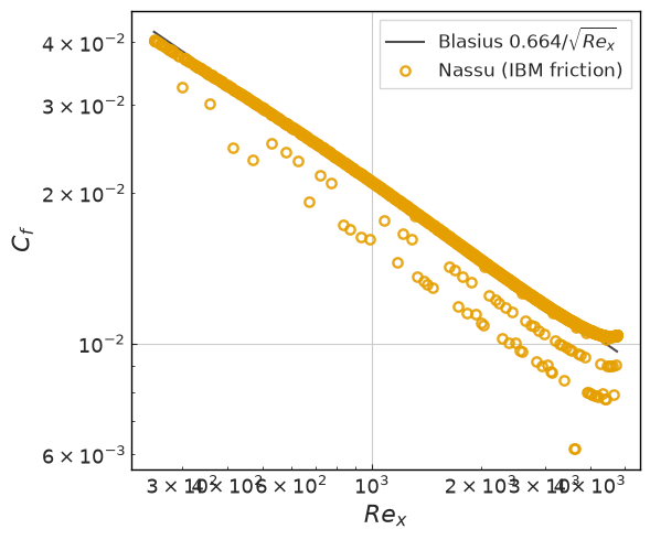
read_body_friction loads the per-triangle traction time series and the static centroid / normal / area topology. We time-average the traction over the settled steady window (time_mean_friction), then take the wall-tangential magnitude per triangle as the wall-shear stress and form Cf = tau_w / (0.5 rho U_inf^2) (skin_friction_coefficient). Each triangle’s centroid x maps to a local Re_x = U_inf (x - x_le) / nu.

Only the resolved interior of the plate is compared: the leading-edge singularity (Cf -> inf as Re_x -> 0) and the IBM smearing over the first ~2-3 fine cells make x very close to the leading edge unreliable, so we restrict the overlay to 0.05 L <= x - x_le <= 0.95 L.

[ ]:

import nassu.viz as common

common.use_style()

bf = common.read_body_friction(sim_cfg, "plate", series="friction")

# Time-mean traction over the settled window (drop the first half as transient).
stats_start = 0.5 * sim_cfg.n_steps
t_mean = common.time_mean_friction(bf, stats_start=stats_start)

# Per-triangle wall-shear stress and skin-friction coefficient.
tau_w = common.wall_shear_stress(t_mean, bf.normal)
cf_tri = common.skin_friction_coefficient(t_mean, bf.normal, rho_ref=rho_inf, u_ref=u_inf)

# Map each triangle centroid to its local Reynolds number.
x_local = bf.centroid[:, 0] - x_le
Re_x_tri = u_inf * x_local / nu

# Restrict to the resolved, singularity-free interior of the plate.
mask = (x_local >= 0.05 * plate_length) & (x_local <= 0.95 * plate_length)
order = np.argsort(x_local[mask])
Re_x_s = Re_x_tri[mask][order]
cf_s = cf_tri[mask][order]
print(f"{mask.sum()} of {bf.n_tri} triangles in the comparison window")

`Cf(x)` vs Blasius¶

The per-triangle simulated Cf (there are many triangles at each x across the span; they collapse onto a single curve for a 2-D boundary layer) overlaid on the Blasius 0.664 / sqrt(Re_x) line.

[ ]:

import matplotlib.pyplot as plt

fig, ax = common.fig_single()

# Blasius reference over the sampled Re_x range.
Re_ref = np.linspace(max(Re_x_s.min(), 1.0), Re_x_s.max(), 200)
ax.plot(
    Re_ref,
    blasius_cf(Re_ref),
    **common.markers.exp_line(linestyle="-"),
    label="Blasius $0.664/\\sqrt{Re_x}$",
)

# Simulated per-triangle Cf from the body_nodes friction export.
ax.plot(Re_x_s, cf_s, **common.markers.sim(shape="o"), label="Nassu (IBM friction)")

ax.set_xlabel("$Re_x$")
ax.set_ylabel("$C_f$")
ax.set_xscale("log")
ax.set_yscale("log")
ax.legend()
plt.tight_layout()
plt.show(fig)

Relative error along the plate¶

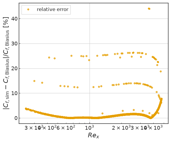
The pointwise relative error |Cf_sim - Cf_blasius| / Cf_blasius against the analytical curve. We expect the error to be largest near the leading edge (thin, under-resolved boundary layer plus IBM smearing) and to settle to a few percent over the bulk of the plate.

[ ]:

cf_blasius_s = blasius_cf(Re_x_s)
rel_err = np.abs(cf_s - cf_blasius_s) / cf_blasius_s

fig, ax = common.fig_single()
ax.plot(Re_x_s, 100 * rel_err, **common.markers.sim(shape="."), label="relative error")
ax.set_xlabel("$Re_x$")
ax.set_ylabel(r"$|C_{f,\mathrm{sim}} - C_{f,\mathrm{Blasius}}| / C_{f,\mathrm{Blasius}}$ [%]")
ax.set_xscale("log")
ax.legend()
plt.tight_layout()
plt.show(fig)

print(f"median relative error over the comparison window: {100 * np.median(rel_err):.1f}%")

Summary¶

Success criteria for this validation case:

The simulated local skin-friction coefficient Cf(x) collapses onto the Blasius 0.664 / sqrt(Re_x) curve across the resolved plate (0.05 L <= x <= 0.95 L).
The median pointwise relative error over the comparison window is within a few percent.
The error grows toward the leading edge, consistent with the thin, less-resolved boundary layer there and the diffuse-interface IBM smearing of the wall - a documented limit of the method, not a solver error.

The case is the canonical flat-wall counterpart to 01_flow_over_sphere: it validates the data.body_nodes friction export (issue #879) on a geometry where the per-triangle traction reduces to a pure, analytically known wall-shear stress.

Version¶

[ ]:

sim_info = sim_cfg.output.read_info()
print("Version:", sim_info["version"])
print("Commit hash:", sim_info["commit"])

Configuration¶

[ ]:

from IPython.display import Code

Code(filename=filename)