Solving the TBL equation

The thin boundary layer model leaves us with a second-order ordinary differential equation for the tangential velocity along the wall normal. This page works through its discretization on the wall-normal stencil and its solution by the tridiagonal matrix algorithm (TDMA), ending with the recovery of the friction velocity that the wall model feeds back to the solver.

Finite-difference stencil

The distance \(h_{\mathrm{wm}}\) between \(\mathrm{P_{0}}\) and \(\mathrm{P_{N}}\) is divided in \(N\) points to which the simplified TBL equation is solved through a finite difference scheme:

(1)\[ \left[\nu_{\mathrm{T}}-\frac{h_{\mathrm{wm}}}{2N}\frac{\partial \nu_{\mathrm{T}}}{\partial x_{n}}\right]^{\left(i\right)}u_{t}^{\left(i-1\right)} - 2\nu_{\mathrm{T}}^{\left(i\right)}u_{t}^{\left(i\right)}+\left[\nu_{\mathrm{T}}+\frac{h_{\mathrm{wm}}}{2N}\frac{\partial \nu_{\mathrm{T}}}{\partial x_{n}}\right]^{\left(i\right)}u_{t}^{\left(i+1\right)} = \left(\frac{h_{\mathrm{wm}}}{N}\right)^{2}\frac{1}{\rho}\frac{\partial p}{\partial x_{t}}^{(i)} \]

where \(\nu_{\mathrm{T}}=\nu+\nu_{\mathrm{e}}\)

(2)\[ \frac{\partial \nu_{\mathrm{T}}}{\partial x_{n}}=\kappa u^{*}\left[1-\frac{2\left(A^{+}-x_{n}^{+}\right)}{A^{+}}e^{-\frac{x_{n}^{+}}{A^{+}}}+\frac{\left(A^{+}-2x_{n}^{+}\right)}{A^{+}}e^{-\frac{2x_{n}^{+}}{A^{+}}}\right] \]

The \(\nu\) factor in \(\nu_{\mathrm{e}}\) cancels because the derivative is taken with respect to the physical wall-normal coordinate \(x_{n}\) while \(\nu_{\mathrm{e}}\) is expressed in wall units \(x_{n}^{+}=x_{n}u^{*}/\nu\), which is why the prefactor reduces to \(\kappa u^{*}\).

The value for \(x_{n}^{+}\) in a \(i\) point is then \(x_{n}^{+}=\left(h_{\mathrm{wm}}i/N\right)\left(u^{*}/\nu\right)\).

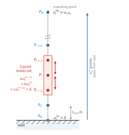
The wall-normal grid for the thin-boundary-layer solve. The TBL equation is discretised on N points from the wall \(\mathrm{P_0}\) to the matching point \(\mathrm{P_N}\); a three-point finite-difference molecule at an interior point couples it to its neighbours, producing the tridiagonal system solved by the TDMA.

Equilibrium vs non-equilibrium: the pressure-gradient term

This one term decides which model you are running. Setting \(\partial p / \partial x_{t} = 0\) gives the equilibrium model, valid where the streamwise pressure gradient is small. Retaining it gives the non-equilibrium model, the one to use wherever that gradient is not negligible: separation, reattachment, and adverse-pressure-gradient regions.

The equilibrium lattice-BC solve described on this page sets \(\partial p / \partial x_{t} = 0\), so the source terms \(d_{\left(i\right)}\) vanish. The non-equilibrium model evaluates a single tangential pressure gradient per node by central-differencing the LBM density along the local tangential direction, and applies it uniformly across the interior rows. Since \(p = \rho c_{s}^{2}\),

(3)\[ \frac{\partial p}{\partial x_{t}}= \frac{\left[\rho\left(x_{t}+\Delta x_{t}\right)-\rho\left(x_{t}-\Delta x_{t}\right)\right]c_{s}^{2}}{2\Delta x_{t}} \]

Tridiagonal system and TDMA

The set of velocity equations generated can be solved with a TDMA (tridiagonal matrix algorithm) to which the velocity equation may be written as:

(4)\[ a_{\left(i\right)}u^{\left(i-1\right)} + b_{\left(i\right)}u^{\left(i\right)} + c_{\left(i\right)}u^{\left(i+1\right)} = d_{\left(i\right)} \]

since \(u^{\left(0\right)}=0\), \(a_{1}=0\) and:

(5)\[ a_{\left(i\right)} = \left[\nu_{\mathrm{T}}-\frac{h_{\mathrm{wm}}}{2N}\frac{\partial \nu_{\mathrm{T}}}{\partial x_{n}}\right]^{\left(i\right)} \]

(6)\[ b_{\left(i\right)} = -2\nu_{\mathrm{T}}^{\left(i\right)} \]

(7)\[ c_{\left(i\right)} = \left[\nu_{\mathrm{T}}+\frac{h_{\mathrm{wm}}}{2N}\frac{\partial \nu_{\mathrm{T}}}{\partial x_{n}}\right]^{\left(i\right)} \]

(8)\[ d_{\left(i\right)} = \left(\frac{h_{\mathrm{wm}}}{N}\right)^{2}\frac{1}{\rho}\frac{\partial p}{\partial x_{t}}^{(i)} \]

For \(2\leq i \leq N-1\). We consider that \(u^{\left(N\right)}=u_{t,\mathrm{P_{N}}}\) and \(c_{\left(N-1\right)}=0\), hence:

(9)\[ d_{\left(N-1\right)} = \left(\frac{h_{\mathrm{wm}}}{N}\right)^{2}\frac{1}{\rho}\frac{\partial p}{\partial x_{t}}^{\left(N-1\right)} - \left[\nu_{\mathrm{T}}+\frac{h_{\mathrm{wm}}}{2N}\frac{\partial \nu_{\mathrm{T}}}{\partial x_{n}}\right]^{\left(N-1\right)}u_{t,\mathrm{P_{N}}} \]

The matrix of a linear system is then written as:

\[\begin{split} \begin{bmatrix} b_{\left(1\right)} & c_{\left(1\right)} & 0 & 0 & \cdots & 0 & 0 \\ a_{\left(2\right)} & b_{\left(2\right)} & c_{\left(2\right)} & 0 & \cdots & 0 & 0 \\ 0 & a_{\left(3\right)} & b_{\left(3\right)} & c_{\left(3\right)} & \cdots & 0 & 0 \\ 0 & 0 & a_{\left(4\right)} & b_{\left(4\right)} & \cdots & 0 & 0 \\ 0 & 0 & 0 & \cdots & a_{\left(N-2\right)} & b_{\left(N-2\right)} & c_{\left(N-2\right)} \\ 0 & 0 & 0 & \cdots & 0 & a_{\left(N-1\right)} & b_{\left(N-1\right)} \end{bmatrix} \begin{bmatrix} u^{\left(1\right)} \\ u^{\left(2\right)} \\ u^{\left(3\right)} \\ u^{\left(4\right)} \\ \vdots \\ u^{\left(N-1\right)} \end{bmatrix} = \begin{bmatrix} d_{\left(1\right)} \\ d_{\left(2\right)} \\ d_{\left(3\right)} \\ d_{\left(4\right)} \\ \vdots \\ d_{\left(N-1\right)} \end{bmatrix} \end{split}\]

For the first term, \(i=1\):

(10)\[ c_{\left(1\right)}^{'}=\frac{c_{\left(1\right)}}{b_{\left(1\right)}} \]

(11)\[ d_{\left(1\right)}^{'}=\frac{d_{\left(1\right)}}{b_{\left(1\right)}} \]

After which, the following coefficients up to \(N-1\) are calculated:

(12)\[ c_{\left(i\right)}^{'}=\frac{c_{\left(i\right)}}{b_{\left(i\right)}-a_{\left(i\right)}c_{\left(i-1\right)}^{'}} \]

(13)\[ d_{\left(i\right)}^{'}=\frac{d_{\left(i\right)}-a_{\left(i\right)}d_{\left(i-1\right)}^{'}}{b_{\left(i\right)}-a_{\left(i\right)}c_{\left(i-1\right)}^{'}} \]

Knowing that \(u_{t}^{\left(N\right)}=u_{t,\mathrm{P_{N}}}\), the remaining velocities are calculated backwards by:

\[ u_{t}^{\left(i\right)}=d_{\left(i\right)}^{'}-c_{\left(i\right)}^{'}u_{t}^{\left(i+1\right)} \]

Along these lines, the friction velocity can be calculated with a second-order finite-difference scheme:

(14)\[ u^{*}=\sqrt{\nu \frac{\left(-3u_{t}^{(0)}+4 u_{t}^{(1)}-u_{t}^{(2)}\right)}{2 h_{\mathrm{wm}}/N}} \]

Wall-clustered grid

The stencil above places the \(N\) points at a uniform physical spacing \(h_{\mathrm{wm}}/N\). Because the wall model is driven by the wall-normal gradient at \(\mathrm{P_0}\), resolution is best spent near the wall. Nassu therefore allows the grid to be clustered toward the wall while keeping the tridiagonal (Thomas) solver untouched: the spacing variation is absorbed into a coordinate map, not a wider stencil.

The solve is carried out on a uniform computational coordinate \(\xi \in \left[0, 1\right]\) with constant spacing \(\Delta\xi = 1/N\), related to the physical wall-normal distance \(x_n\) by an exponential map clustered at the wall (\(\xi = 0\)):

(15)\[ x_{n}\left(\xi\right) = h_{\mathrm{wm}}\,\frac{e^{\beta\xi}-1}{e^{\beta}-1}, \qquad J\left(\xi\right) \equiv \frac{\mathrm{d}x_{n}}{\mathrm{d}\xi} = h_{\mathrm{wm}}\,\frac{\beta\, e^{\beta\xi}}{e^{\beta}-1} \]

The clustering strength \(\beta \ge 0\) is the TDMA_stretch_beta parameter (default \(\beta = 2\), which places the first node inside the viscous sublayer for a typical near-wall cell of 10-50 wall units); \(\beta \to 0\) recovers the uniform grid \(x_n = h_{\mathrm{wm}}\,\xi\) with \(J = h_{\mathrm{wm}}\), and the wall-unit position becomes \(x_{n}^{+}=x_{n}\left(\xi_i\right)\left(u^{*}/\nu\right)\) in (2).

Rather than expand the variable-coefficient operator, the TBL equation is discretised in its conservative form. Mapping \(\partial_{x_n}\!\left(\nu_{\mathrm{T}}\,\partial_{x_n} u_t\right)\) into \(\xi\) gives

(16)\[ \frac{\partial}{\partial \xi}\!\left(\frac{\nu_{\mathrm{T}}}{J}\frac{\partial u_t}{\partial \xi}\right) = J\,\frac{1}{\rho}\frac{\partial p}{\partial x_{t}} \]

A finite-volume balance on the uniform \(\xi\)-grid, with the flux coefficient \(\Gamma = \nu_{\mathrm{T}}/J\) evaluated at the cell faces \(i\pm\tfrac{1}{2}\), keeps the system tridiagonal:

(17)\[ a_{\left(i\right)} = \Gamma_{i-\frac{1}{2}}, \qquad b_{\left(i\right)} = -\left(\Gamma_{i-\frac{1}{2}}+\Gamma_{i+\frac{1}{2}}\right), \qquad c_{\left(i\right)} = \Gamma_{i+\frac{1}{2}}, \qquad d_{\left(i\right)} = \Delta\xi^{2}\,J^{\left(i\right)}\,\frac{1}{\rho}\frac{\partial p}{\partial x_{t}}^{\left(i\right)} \]

The face viscosity \(\nu_{\mathrm{T}}\) in \(\Gamma_{i\pm\frac{1}{2}}\) is the van Driest value at the face wall-distance. The conservative form absorbs the \(\partial\nu_{\mathrm{T}}/\partial x_n\) term that appears explicitly in (5)-(7), so no separate eddy-viscosity-derivative coefficient is needed. The forward/backward Thomas sweeps (12)-(13) are identical; only the coefficient assembly changes. The friction velocity (14) carries the metric at the wall,

(18)\[ u^{*}=\sqrt{\nu\,\frac{\left(-3u_{t}^{(0)}+4 u_{t}^{(1)}-u_{t}^{(2)}\right)}{2\,\Delta\xi\,J\left(0\right)}} \]

which reduces to (14) for \(\beta \to 0\) since \(\Delta\xi\,J\left(0\right) = h_{\mathrm{wm}}/N\).