Couette (Startup)

The simulation of a Couette flow is mainly used for validation of the transient flow description through the current collision operator implemented. In this case, the moving wall boundary condition is employed at the \(y=h\) and the halfway bounce-back BC \(y=0\), those BC are therefore also validated.

from nassu.cfg.model import ConfigScheme

filename = "validation/analytical/01_couette_flow/01_couette_flow.nassu.yaml"

sim_cfgs = ConfigScheme.sim_cfgs_from_file_dct(filename)

The simulation parameters are shown below

import pandas as pd
from IPython.display import HTML

sim_cfg = sim_cfgs["startupCouette", 0]
dct = {
    "NX": [sim_cfg.domain.domain_size.x],
    "NY": [sim_cfg.domain.domain_size.y],
    "tau": [sim_cfg.models.LBM.tau],
    "time_steps": sim_cfg.n_steps,
}
df = pd.DataFrame(dct, index=None)

HTML(df.to_html())

	NX	NY	tau	time_steps
0	32	32	0.9	4000

Results

The plots of the evolution of velocity profile compared with the analytical solution are shown below

import matplotlib.pyplot as plt
import numpy as np

import nassu.viz as common
from nassu.cfg.schemes.simul import SimulationConfigs
from nassu.viz.analysis import couette_adimensional_time, couette_startup_velocity

common.use_style()

The startup-Couette analytical reference (steady and transient profiles, adimensional time) lives in nassu.viz.analysis and is unit-tested; the notebook only reads the exported profile and overlays it against that reference.

def post_proc_couette_time_step(sim_cfg: SimulationConfigs, time_step: int, ax):
    line = sim_cfg.output.exports["default_series"].series.lines["velocity_profile"]

    points_df = pd.read_csv(line.points_filename)
    data_df = line.read_full_data("ux")

    u_wall = sim_cfg.models.BC.BC_map[0].params["ux"]
    nu = sim_cfg.models.LBM.kinematic_viscosity
    h = sim_cfg.domain.domain_size.y
    adim_time = couette_adimensional_time(nu, h, time_step)
    ax.set_title(r"Couette $\nu u/h^2=$" + f"{adim_time:.4f}")

    x_abs = points_df["y"].to_numpy(dtype=np.float32)
    x = (x_abs) / (len(x_abs) - 1)
    num_y = data_df[data_df["time_step"] == time_step]
    num_y = num_y.drop(columns="time_step").to_numpy().T
    ax.plot(x, num_y, **common.markers.sim(), label="AeroSim")

    analytical_y = couette_startup_velocity(u_wall, x, adim_time)
    ax.plot(x, analytical_y, **common.markers.exp_line(linestyle="--"), label="Analytical")

Process velocity profiles for some time steps

fig, ax = plt.subplots(2, 2, figsize=(12, 9))

time_steps_proc = [80, 400, 800, 4000]
ax_ticks = [0, 0.0005, 0.001, 0.0015, 0.002]
ax_ticks_label = [f"{x:4.1e}" for x in ax_ticks]
for idx, t in enumerate(time_steps_proc):
    i, j = idx % 2, idx // 2
    post_proc_couette_time_step(sim_cfg, t, ax[i, j])
    ax[i, j].set_yticks(ax_ticks)
    ax[i, j].set_yticklabels(ax_ticks_label)
    ax[i, j].legend()

plt.tight_layout()
plt.show(fig)

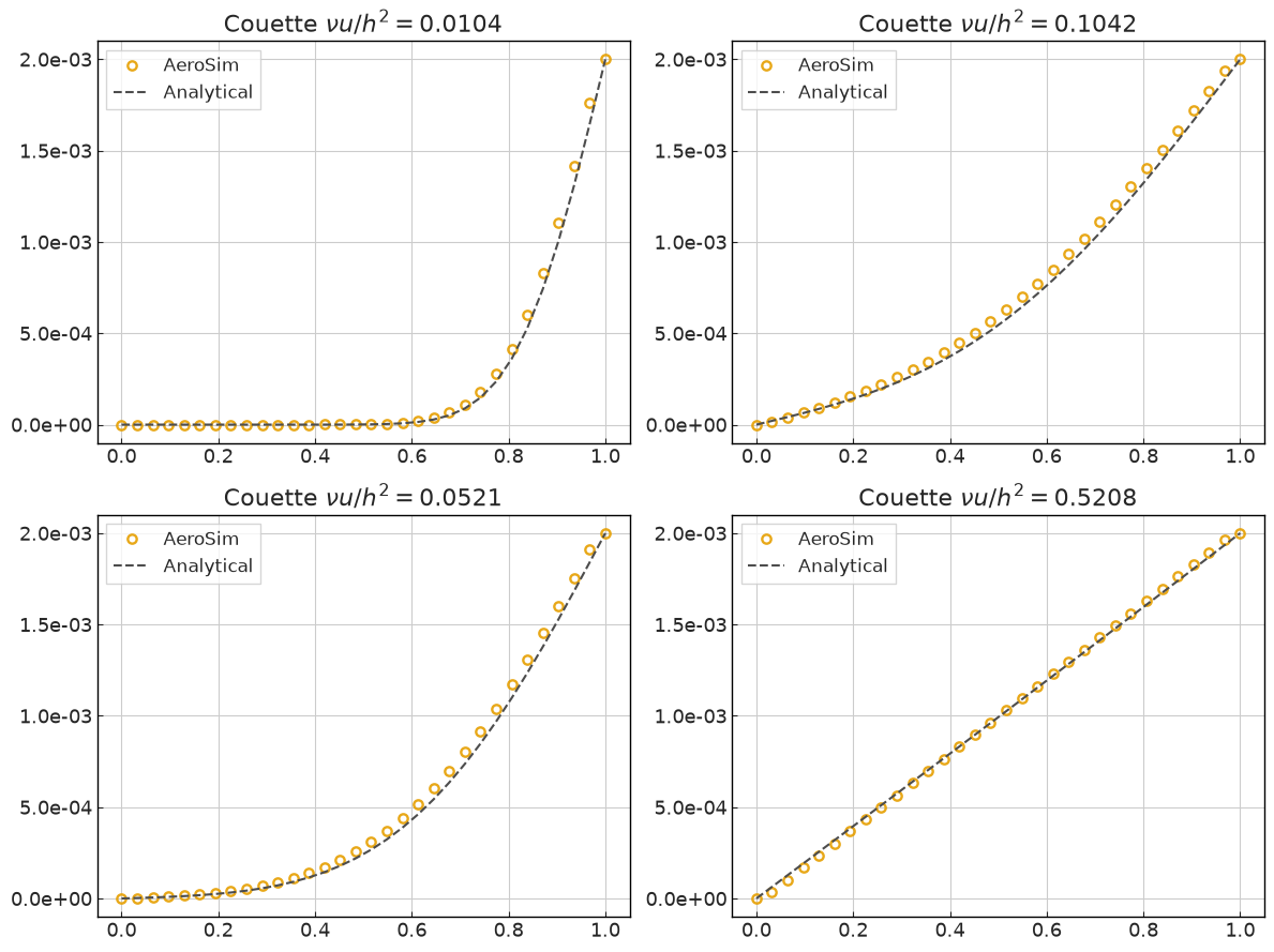
The walls have a slight inaccuracy due to the halfway bounce-back not being “rightly” implemented in moments representation.

Despite that, results show a very satisfatory agreement between numerical model and analytical solution, confirming the solver capability to represent a transient flow.

Version

sim_info = sim_cfg.output.read_info()

nassu_commit = sim_info["commit"]
nassu_version = sim_info["version"]
print("Version:", nassu_version)
print("Commit hash:", nassu_commit)

Version: 2.0.0a7
Commit hash: 5e47f2762575c2d285254d36bfd354b6af09fda1

Configuration

from IPython.display import Code

Code(filename=filename)

simulations:
  - name: startupCouette
    save_path: ./validation/analytical/01_couette_flow/results/startup_couette

    n_steps: 4000

    report:
      frequency: 500

    domain:
      domain_size:
        x: 32
        y: 32
      block_size: 8

    data:
      monitors:
        fields:
          macrs_stats:
            macrs: [rho, u]
            stats: [min, max, mean, pos]
            interval: {frequency: 100}
      exports:
        default:
          macrs: [rho, u]
          interval:
            frequency: 80
            lvl: 0
          target:
            volumes:
              default: {}
          outputs:
            instantaneous: true
        default_series:
          macrs: [rho, u]
          interval: {frequency: 80, lvl: 0}
          target:
            lines:
              velocity_profile:
                dist: 1
                start_pos: [4, 0]
                end_pos: [4, 32]
          outputs:
            instantaneous: true

    models:
      precision:
        default: single

      LBM:
        tau: 0.9
        vel_set: D2Q9
        coll_oper: RRBGK

      engine:
        name: CUDA

      BC:
        periodic_dims: [true, false]
        BC_map:
          - pos: N
            BC: RegularizedVelocityWall
            wall_normal: N
            params:
              ux: 2e-3
              uy: 0
          - pos: S
            BC: RegularizedVelocityWall
            wall_normal: S
            params:
              ux: 0
              uy: 0