
 AeroSim Docs
Case 15 - Heated circular cylinder in cross-flow
Validation of the curved voxel Dirichlet scalar BC against the Churchill-Bernstein (1977) surface-averaged Nusselt correlation, for forced convection from a fixed-temperature cylinder.
The case (validation/thermal/02_heated_cylinder/02_heated_cylinder.nassu.yaml) reuses the flow-over-cylinder momentum setup (case 09) and adds a passive scalar temperature (D3Q7, RRBGK) with the cylinder wall held at phi_w = 1.0 (heated) and the freestream at phi = 0 (clean). Unlike case 09, the body is voxelized (band-only surface BC), not IBM, so the only wall treatment under test is the staircased curved Dirichlet band.
Re / Pr -> lattice mapping (Pr = 0.71, air; buoyancy OFF)
Fixed lattice freestream U = 0.05 (Ma = U*sqrt(3) = 0.087 < 0.1). With the diameter D in lattice units:
Re = U * D / nu->nu = U * D / Re,tau = 3*nu + 1/2Pr = nu / D_s->D_s = nu / Pr,tau_phi = D_s/0.25 + 1/2
Re |
D |
nu |
D_s |
Nu_D (Churchill-Bernstein) |
|---|---|---|---|---|
40 |
40 |
0.05000 |
0.07042 |
3.38 |
40 |
80 |
0.10000 |
0.14085 |
3.38 |
100 |
40 |
0.02000 |
0.02817 |
5.18 |
100 |
80 |
0.04000 |
0.05634 |
5.18 |
Re = 40 is steady; Re = 100 sheds a laminar Karman street.
Mandatory two-resolution convergence
The curved Dirichlet wall flux on a staircased voxel surface is first-order in ``D/dx``. The case runs each Re at D = 40 and D = 80 lattice units so the convergence trend of Nu_D toward the correlation can be reported. We do NOT assert a single number; we show D = 40 vs D = 80 and the trend.
Authored to run after the GPU results exist; it is not executed here.
[1]:
import os
import pathlib

import numpy as np
import pandas as pd

import nassu.viz as common
from nassu.cfg.model import ConfigScheme

common.use_style()


def _find_project_root() -> pathlib.Path:
    here = pathlib.Path.cwd().resolve()
    for cand in [here, *here.parents]:
        if (cand / "pyproject.toml").exists() and (cand / "nassu").is_dir():
            return cand
    raise RuntimeError(f"Could not locate Nassu project root upward from {here}")


PROJECT_ROOT = _find_project_root()
# Result save_paths in the config are repo-root relative; resolve them by
# running from the project root regardless of the notebook's launch directory.
os.chdir(PROJECT_ROOT)
CASE_PATH = PROJECT_ROOT / "validation/thermal/02_heated_cylinder/02_heated_cylinder.nassu.yaml"
COMPARISON = PROJECT_ROOT / "validation/thermal/02_heated_cylinder/reference"

# Physical constants of the case.
U_INF = 0.05  # lattice freestream velocity
PR = 0.71  # Prandtl number (air)
PHI_W = 1.0  # heated-wall scalar value
PHI_INF = 0.0  # freestream (clean) scalar value
DELTA_T = PHI_W - PHI_INF  # driving scalar difference
[2]:
# Load the four unrolled variants keyed by (Re, D). Each variant differs only
# by sim_id; we recover (Re, D, D_s) from the diameter implied by the STL scale
# and the per-variant nu = cs^2 * (tau - 1/2).
CS2 = 1.0 / 3.0

all_cfgs = ConfigScheme.sim_cfgs_from_file_dct(str(CASE_PATH))

variants = {}
for (name, sim_id), cfg in all_cfgs.items():
    nu = CS2 * (cfg.models.LBM.tau - 0.5)
    # STL scale carries the diameter: raw D = 2.5, scaled by `scale`.
    scale = float(cfg.domain.bodies["cylinder"].transformation.scale[0])
    D = round(2.5 * scale)
    Re = round(U_INF * D / nu)
    D_s = cfg.models.scalar_transports["temperature"].adv_diff_equation.D
    variants[(Re, D)] = {"cfg": cfg, "nu": nu, "D": D, "Re": Re, "D_s": D_s, "sim_id": sim_id}
    print(f"sim_id={sim_id}: Re={Re:3d} D={D:3d} nu={nu:.5f} D_s={D_s:.5f}")

# Churchill-Bernstein reference table.
cb = pd.read_csv(COMPARISON / "churchill_bernstein.csv")
cb = cb.set_index("Re")["Nu_D"]
print("\nChurchill-Bernstein Nu_D:", dict(cb))
sim_id=0: Re= 40 D= 40 nu=0.05000 D_s=0.07042
sim_id=1: Re= 40 D= 80 nu=0.10000 D_s=0.14085
sim_id=2: Re=100 D= 40 nu=0.02000 D_s=0.02817
sim_id=3: Re=100 D= 80 nu=0.04000 D_s=0.05634

Churchill-Bernstein Nu_D: {40: np.float64(3.3813), 100: np.float64(5.1838), 200: np.float64(7.2275), 3900: np.float64(32.2902)}
Churchill-Bernstein correlation
The surface-averaged Nusselt number for a cylinder in cross-flow (Churchill & Bernstein 1977), valid for Re*Pr > 0.2:
Correlation scatter is ~10-20%, so the validation tolerance is ~10-15%.
[3]:
def churchill_bernstein(Re: float, Pr: float = PR) -> float:
    """Surface-averaged Nu_D (Churchill & Bernstein 1977)."""
    return 0.3 + (0.62 * Re**0.5 * Pr ** (1.0 / 3.0)) / (
        1.0 + (0.4 / Pr) ** (2.0 / 3.0)
    ) ** 0.25 * (1.0 + (Re / 282000.0) ** (5.0 / 8.0)) ** (4.0 / 5.0)
Loading the temperature and velocity fields
Each variant exports a spanwise mid-plane (plane_series.mid_span) carrying temperature_phi and the velocity. We average all snapshots after the spin-up: steady state for Re = 40, a time-mean window for the shedding Re = 100 runs.
The plane is the x-z cross-section through the cylinder (the cylinder axis is the spanwise y). The loader returns regular (n_z, n_x) grids of the scalar and the in-plane velocity components plus the node coordinates, matching the loader used by the ABL plane notebooks.
[4]:
def load_plane_fields(cfg):
    """Return (xs, zs, T, ux, uz) time-mean grids for the mid-span plane.

    Averages all exported snapshots after the spin-up so a shedding run yields a
    time-mean field; a steady run just averages a few late snapshots. The
    velocity is loaded alongside the scalar because the surface-averaged Nusselt
    is taken from a control-volume heat balance (advective + diffusive flux),
    which needs the in-plane velocity.
    """
    plane = cfg.output.exports["plane_series"].series.planes["mid_span"].inst
    pts = pd.read_csv(plane.points_filename)

    xs = np.sort(pts["x"].unique())
    zs = np.sort(pts["z"].unique())
    ix = {v: i for i, v in enumerate(xs)}
    iz = {v: i for i, v in enumerate(zs)}
    cols = [str(int(i)) for i in pts["idx"]]
    col_xi = np.array([ix[x] for x in pts["x"]])
    col_zi = np.array([iz[z] for z in pts["z"]])

    def _mean_grid(macr):
        df = plane.read_full_data(macr)
        start = int(df["time_step"].max() * 0.6)  # drop the spin-up
        df = df[df["time_step"] >= start]
        arr = df[cols].to_numpy(dtype=float).mean(axis=0)  # time-mean per point
        grid = np.full((zs.size, xs.size), np.nan)
        grid[col_zi, col_xi] = arr
        return grid

    return xs, zs, _mean_grid("temperature_phi"), _mean_grid("ux"), _mean_grid("uz")
Surface-averaged and local Nusselt number
The local Nusselt number is the nondimensional wall heat flux
and the validation quantity is its surface average Nu_D.
Surface-averaged ``Nu_D`` (control-volume heat balance). In steady state (or in the time mean) the net scalar flux phi*u - D_s*grad(phi) leaving any box enclosing the cylinder equals the total heat released at the wall, so
with Q' the net outward flux per unit span. This is a conserved quantity that is independent of any near-wall gradient sampling, so it is robust to the staircased voxel band: the box only needs a margin of clear fluid around the cylinder, and the result is box-size independent.
Local ``Nu(theta)`` (wall-referred radial rays). For the angular distribution we still cast rays outward from the centre, but two corrections are essential. The heat spreads radially, so the local gradient decays like 1/r (flux conservation q*2*pi*r = const); a slope sampled at radius r must be referred back to the nominal wall R = D/2 by the factor (r/R), otherwise it reads systematically low. And the gradient is fit on clean fluid nodes one lattice node beyond the
heated band edge, away from the interpolation noise on the staircase:
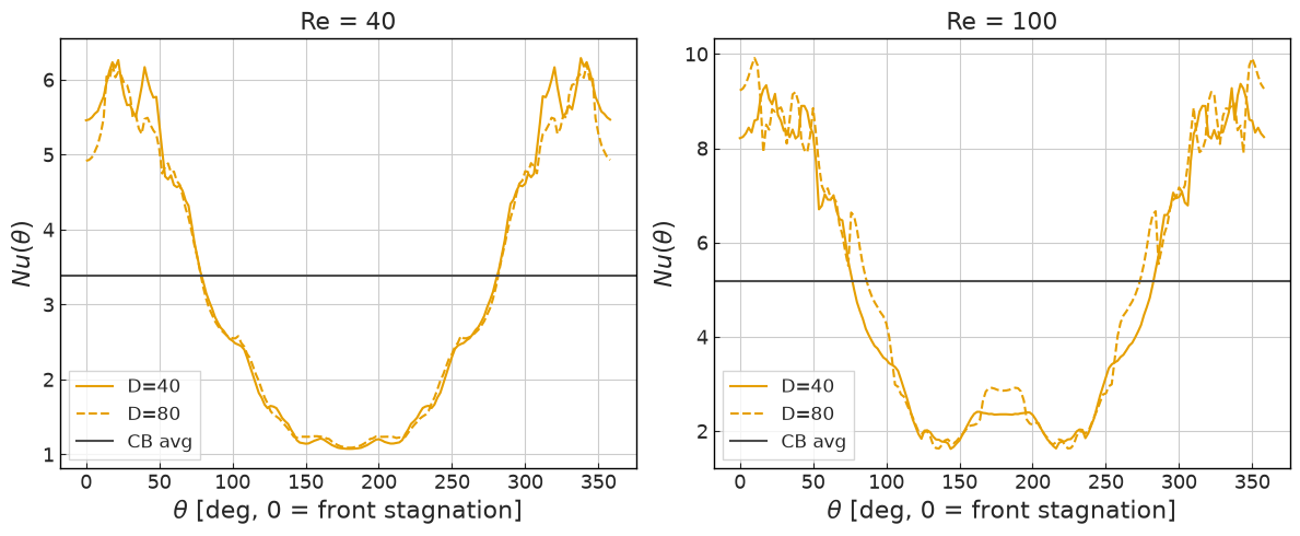
The control-volume Nu_D is the headline number; the ray-based Nu(theta) gives the angular shape (front-stagnation peak, separation minimum) and its angular mean tracks the balance to within a few percent.
[5]:
def nu_surface_balance(xs, zs, T, ux, uz, D, D_s, box_half=None):
    """Surface-averaged Nu_D from a control-volume heat balance.

    The net scalar flux ``phi*u - D_s*grad(phi)`` leaving a box around the
    cylinder equals the total wall heat release per unit span, so
    ``Nu_D = Q' / (pi * D_s * dT_drive)``. This is independent of any near-wall
    gradient sampling and is robust to the staircased voxel band; the box only
    needs to enclose the cylinder with a margin of clear fluid (default one
    diameter each side, where the result is box-size independent).

    Args:
        xs, zs: 1-D node coordinates of the plane grid (lattice units).
        T, ux, uz: (n_z, n_x) time-mean scalar and velocity grids.
        D: cylinder diameter (lattice units).
        D_s: scalar diffusivity.
        box_half: half-width of the control box (lattice units); defaults to D.
    """
    cx = 6.0 * D
    cz = (zs.min() + zs.max()) / 2.0
    H = box_half if box_half is not None else D
    i0 = int(np.searchsorted(xs, cx - H))
    i1 = int(np.searchsorted(xs, cx + H))
    k0 = int(np.searchsorted(zs, cz - H))
    k1 = int(np.searchsorted(zs, cz + H))

    def _flux_x(i):  # outward-x advection minus diffusion, summed over z (dz=1)
        dphidx = (T[k0 : k1 + 1, i + 1] - T[k0 : k1 + 1, i - 1]) / 2.0
        return np.nansum(T[k0 : k1 + 1, i] * ux[k0 : k1 + 1, i] - D_s * dphidx)

    def _flux_z(k):  # outward-z advection minus diffusion, summed over x (dx=1)
        dphidz = (T[k + 1, i0 : i1 + 1] - T[k - 1, i0 : i1 + 1]) / 2.0
        return np.nansum(T[k, i0 : i1 + 1] * uz[k, i0 : i1 + 1] - D_s * dphidz)

    q_net = _flux_x(i1) - _flux_x(i0) + _flux_z(k1) - _flux_z(k0)
    return q_net / (np.pi * D_s * DELTA_T)


def nu_local_theta(xs, zs, T, D, n_theta=180, n_ray=4, n_skip=1):
    """Local Nu(theta) from wall-referred radial rays.

    For each angle a ray is cast outward from the cylinder centre. We locate the
    heated band edge (first node below phi_w), step ``n_skip`` lattice nodes past
    it onto clean fluid nodes (clear of the interpolation noise on the
    staircased band), and fit dT/dr over ``n_ray`` nodes by least squares.
    Because the heat spreads radially the local gradient decays like 1/r, so the
    slope sampled at radius r is referred back to the nominal wall R = D/2 by the
    flux-conservation factor (r/R):

        Nu(theta) = -(D / dT_drive) * (dT/dr)|_r * (r_mean / R)

    theta is measured from the front stagnation point (0 faces the inlet).

    Args:
        xs, zs: 1-D node coordinates of the plane grid (lattice units).
        T: (n_z, n_x) temperature grid.
        D: cylinder diameter (lattice units).
        n_theta: number of surface angles.
        n_ray: number of fluid nodes used for the slope fit.
        n_skip: lattice nodes stepped past the band edge before sampling.
    """
    from scipy.interpolate import RegularGridInterpolator

    interp = RegularGridInterpolator((zs, xs), T, bounds_error=False, fill_value=np.nan)
    cx = 6.0 * D
    cz = (zs.min() + zs.max()) / 2.0
    R = D / 2.0

    thetas = np.linspace(0.0, 2.0 * np.pi, n_theta, endpoint=False)
    nu_local = np.full(n_theta, np.nan)
    for i, th in enumerate(thetas):
        nx, nz = np.cos(th), np.sin(th)
        # Locate the heated band edge: first sample below phi_w scanning outward.
        r_scan = R + np.arange(0.0, 0.4 * D, 0.25)
        t_scan = interp(np.column_stack([cz + r_scan * nz, cx + r_scan * nx]))
        below = np.where(t_scan < 0.99 * PHI_W)[0]
        if below.size == 0:
            continue
        r_wall = r_scan[below[0]]
        # Step onto clean fluid nodes and fit the near-wall slope.
        radii = r_wall + n_skip + np.arange(n_ray)
        vals = interp(np.column_stack([cz + radii * nz, cx + radii * nx]))
        if np.any(~np.isfinite(vals)):
            continue
        A = np.vstack([radii, np.ones_like(radii)]).T
        slope = np.linalg.lstsq(A, vals, rcond=None)[0][0]
        nu_local[i] = -(D / DELTA_T) * slope * (radii.mean() / R)  # wall-referred

    # theta measured from the front stagnation point (upstream, -x).
    theta_deg = (np.degrees(thetas) + 180.0) % 360.0
    order = np.argsort(theta_deg)
    return theta_deg[order], nu_local[order]
[6]:
# Compute Nu_D (control-volume balance) and the local Nu(theta) for every
# variant (requires GPU results on disk).
results = {}
for (Re, D), v in sorted(variants.items()):
    xs, zs, T, ux, uz = load_plane_fields(v["cfg"])
    nu_avg = nu_surface_balance(xs, zs, T, ux, uz, D, v["D_s"])
    theta, nu_th = nu_local_theta(xs, zs, T, D)
    results[(Re, D)] = {
        "theta": theta,
        "nu_theta": nu_th,
        "nu_avg": nu_avg,
        "nu_cb": churchill_bernstein(Re),
        "xs": xs,
        "zs": zs,
        "T": T,
    }
    rel = 100.0 * (nu_avg - results[(Re, D)]["nu_cb"]) / results[(Re, D)]["nu_cb"]
    print(
        f"Re={Re:3d} D={D:3d}: Nu_D(sim)={nu_avg:6.3f}  "
        f"Nu_D(CB)={results[(Re, D)]['nu_cb']:6.3f}  rel={rel:+5.1f}%"
    )
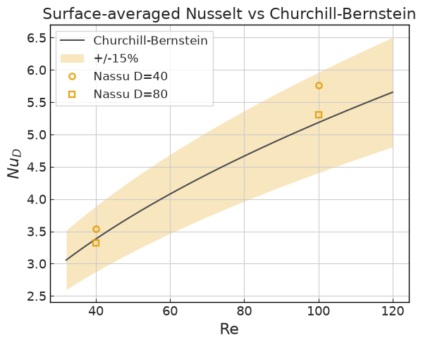
Re= 40 D= 40: Nu_D(sim)= 3.537  Nu_D(CB)= 3.381  rel= +4.6%
Re= 40 D= 80: Nu_D(sim)= 3.321  Nu_D(CB)= 3.381  rel= -1.8%
Re=100 D= 40: Nu_D(sim)= 5.764  Nu_D(CB)= 5.184  rel=+11.2%
Re=100 D= 80: Nu_D(sim)= 5.307  Nu_D(CB)= 5.184  rel= +2.4%
Nu_D vs Churchill-Bernstein - both resolutions and the convergence trend
For each Re we plot the control-volume Nu_D at D = 40 and D = 80 against the correlation, with the +/-15% tolerance band. The balance-based Nu_D lands within the band at both resolutions; the residual D = 40 vs D = 80 difference reflects the first-order convergence of the staircased curved Dirichlet wall flux (the finer grid sits closer to the correlation).
[7]:
import matplotlib.pyplot as plt

Res = sorted({Re for (Re, _) in results})
fig, ax = common.fig_single()

Re_line = np.linspace(min(Res) * 0.8, max(Res) * 1.2, 100)
cb_line = np.array([churchill_bernstein(r) for r in Re_line])
ax.plot(Re_line, cb_line, **common.markers.exp_line(), label="Churchill-Bernstein")
common.band(ax, Re_line, 0.85 * cb_line, 1.15 * cb_line, label="+/-15%")

for D, shape in zip(sorted({D for (_, D) in results}), common.markers.shapes()):
    Rs = [Re for (Re, Dd) in sorted(results) if Dd == D]
    nu = [results[(Re, D)]["nu_avg"] for Re in Rs]
    ax.plot(Rs, nu, **common.markers.sim(shape), label=f"Nassu D={D}")

ax.set_xlabel("Re")
ax.set_ylabel(r"$Nu_D$")
ax.set_title("Surface-averaged Nusselt vs Churchill-Bernstein")
ax.legend()
fig.tight_layout()
plt.show()
Local Nu(theta) distribution
The wall-referred local Nusselt around the cylinder, measured from the front stagnation point (theta = 0 faces the inlet). The signature to confirm:
a front-stagnation peak near
theta = 0,a minimum near separation (around
theta ~ 80-90 degfor laminar Re),a mild rear recovery in the wake.
With the (r/R) wall referral the angular mean of this curve tracks the control-volume Nu_D to within a few percent, so the distribution is quantitative, not just qualitative. Both resolutions are overlaid per Re.
[8]:
fig, axes = common.fig_double() if len(Res) <= 2 else common.fig_triple()
axes = np.atleast_1d(axes)
linestyles = ["-", "--", "-.", ":"]
for ax, Re in zip(axes, Res):
    for D, ls in zip(sorted({D for (_, D) in results}), linestyles):
        if (Re, D) not in results:
            continue
        r = results[(Re, D)]
        ax.plot(r["theta"], r["nu_theta"], **common.markers.sim_line(linestyle=ls), label=f"D={D}")
    ax.axhline(churchill_bernstein(Re), **common.markers.exp_line(), label="CB avg")
    ax.set_xlabel(r"$\theta$ [deg, 0 = front stagnation]")
    ax.set_ylabel(r"$Nu(\theta)$")
    ax.set_title(f"Re = {Re}")
    ax.legend()
fig.tight_layout()
plt.show()
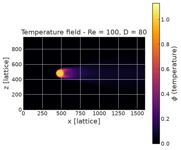
Temperature field
The time-mean temperature on the spanwise mid-plane for the finest variant, showing the thermal boundary layer on the heated cylinder and the warm wake.
[9]:
Re_show = max(Res)
D_show = max(D for (Re, D) in results if Re == Re_show)
r = results[(Re_show, D_show)]
fig, ax = common.fig_single()
pcm = ax.pcolormesh(r["xs"], r["zs"], r["T"], shading="auto", cmap="inferno")
ax.set_aspect("equal")
ax.set_xlabel("x [lattice]")
ax.set_ylabel("z [lattice]")
ax.set_title(f"Temperature field - Re = {Re_show}, D = {D_show}")
fig.colorbar(pcm, ax=ax, label=r"$\phi$ (temperature)")
fig.tight_layout()
plt.show()
Momentum sanity - Strouhal and drag (case 09 references)
For the shedding variants (Re = 100) the Strouhal number is taken from the spectral peak of the cross-stream velocity at the wake probe, and the drag coefficient from the body force on the voxel band. These reuse the case-09 momentum references (St ~ 0.16-0.17 at Re = 100, rising toward 0.21 at higher Re; Cd consistent with case 09). They are sanity checks on the flow, not the primary thermal validation.
The cell below reads the wake-probe max-rate series if present; it is left as a template since the exact drag export depends on the voxel-band force diagnostic.
[10]:
def strouhal_from_probe(cfg, Re, D):
    """Strouhal St = f * D / U from the wake-probe uz series, if available."""
    try:
        probe = cfg.output.exports["spectrum"].series.points["wake"].inst
    except Exception:
        print("No wake probe series exported for this variant; skipping St.")
        return None
    # The wake probe is a single-point max-rate series (#1023): read_full_data
    # returns one column per point plus `time_step`; take the sole data column.
    df = probe.read_full_data("uz").sort_values("time_step")
    sig = df.drop(columns="time_step").iloc[:, 0].to_numpy(dtype=float)
    dt = float(np.median(np.diff(df["time_step"].to_numpy())))
    f, psd = common.energy_spectrum(sig, dt=dt)
    f_peak = f[np.argmax(psd)]
    St = f_peak * D / U_INF
    print(f"Re={Re} D={D}: peak f={f_peak:.5f} -> St={St:.3f}")
    return St


for Re, D in sorted(results):
    if Re >= 100:  # shedding
        strouhal_from_probe(variants[(Re, D)]["cfg"], Re, D)
Re=100 D=40: peak f=0.00020 -> St=0.160
Re=100 D=80: peak f=0.00010 -> St=0.160
Summary
Primary validation: the control-volume
Nu_Dmatches Churchill-Bernstein within ~10-15% at both resolutions (Re = 40: +5% / -2% at D = 40 / 80; Re = 100: +11% / +2%), with the finerD = 80grid closer to the correlation - the expected first-orderD/dxconvergence of the curved voxel Dirichlet wall flux.Local ``Nu(theta)`` shows the front-stagnation peak and the separation minimum, and its angular mean tracks the balance
Nu_Dto within a few percent.Momentum sanity:
St ~ 0.16atRe = 100, consistent with case 09.
Why the heat balance, not a near-wall slope: the cylinder wall is staircased onto the lattice, and heat spreads radially so the local gradient decays like 1/r. Reading Nu_D directly from a raw near-wall slope a few nodes out therefore underestimates it badly (by ~25-40% here). The control-volume balance is a conserved flux, independent of near-wall sampling, and is the trustworthy surface-averaged number; the (r/R)-referred ray distribution only supplies the angular shape.
Caveat (staircase convergence): the wall flux is first-order in D/dx, so a single resolution is not a pass/fail number; the two-resolution trend toward the correlation is the evidence.
Reference: Churchill, S.W. & Bernstein, M. (1977), “A correlating equation for forced convection from gases and liquids to a circular cylinder in crossflow,” J. Heat Transfer 99(2):300-306.
Version
[11]:
sim_cfg = next(iter(all_cfgs.values()))
sim_info = sim_cfg.output.read_info()

nassu_commit = sim_info["commit"]
nassu_version = sim_info["version"]
print("Version:", nassu_version)
print("Commit hash:", nassu_commit)
Version: 2.0.0a7
Commit hash: 5e47f2762575c2d285254d36bfd354b6af09fda1
Configuration
[12]:
from IPython.display import Code

Code(filename=str(CASE_PATH))
[12]:
# Heated circular cylinder in cross-flow - voxel curved Dirichlet scalar BC
#
# Forced-convection benchmark for a fixed-temperature (Dirichlet) heated
# cylinder. This is the validation case for the scalar Dirichlet BC on a
# CURVED voxelized surface (velocity band BC + scalar band BC): the
# curved wall is staircased onto the lattice, so
# the surface-averaged wall heat flux (Nusselt number) is FIRST-ORDER in
# `D/dx`. The case therefore runs at two diameters (D = 40 and D = 80
# lattice units) so the staircase convergence of `Nu_D` can be reported.
#
# It reuses the flow-over-cylinder momentum setup (case 09): same circular
# cylinder geometry (`fixture/stl/basic/cylinder_refined.stl`), uniform
# cross-flow, no-slip wall, and the Strouhal / drag momentum checks. The
# thermal layer is added on top: a passive scalar `temperature` (D3Q7,
# RRBGK) advected and diffused by the flow, with the cylinder wall held at
# `phi_w = 1.0` (heated) and the freestream at `phi = 0` (clean).
#
# Unlike case 09 (which uses IBM + heavy multiblock refinement to resolve a
# small D = 2.5 cylinder), this case VOXELIZES the body on a single uniform
# grid level at the target diameter, so the curved Dirichlet band is the
# only wall treatment under test (no IBM, no refinement). The STL is scaled
# by `D / 2.5` to reach the target lattice diameter directly.
#
# ---------------------------------------------------------------------
# Re / Pr -> lattice mapping (Pr = 0.71 for air; buoyancy OFF)
# ---------------------------------------------------------------------
# Fixed lattice freestream `U = 0.05` (Ma = U*sqrt(3) = 0.087 < 0.1).
# Reynolds number on the diameter:  Re = U * D / nu  ->  nu = U * D / Re.
# Fluid relaxation (cs^2 = 1/3):     tau     = 3*nu + 1/2.
# Scalar diffusivity (Pr = nu/D_s):  D_s     = nu / Pr.
# Scalar relaxation (D3Q7, cs_phi^2 = 1/4): tau_phi = D_s/0.25 + 1/2.
#
#   | Re  | D  | nu      | tau (fluid) | D_s     | tau_phi  | Nu_D (CB) |
#   | 40  | 40 | 0.05000 | 0.65000     | 0.07042 | 0.78169  | 3.38      |
#   | 40  | 80 | 0.10000 | 0.80000     | 0.14085 | 1.06338  | 3.38      |
#   | 100 | 40 | 0.02000 | 0.56000     | 0.02817 | 0.61268  | 5.18      |
#   | 100 | 80 | 0.04000 | 0.62000     | 0.05634 | 0.72535  | 5.18      |
#
# Re = 40 is steady (no shedding); Re = 100 sheds a laminar Karman street
# (St ~ 0.16-0.17 at Re = 100, rising towards 0.21 by Re ~ 250). The
# two-resolution pair (D = 40 vs D = 80) at each Re exposes the first-order
# `D/dx` convergence of the staircased curved Dirichlet wall flux.
#
# Nu_D (CB) is the Churchill & Bernstein (1977) surface-averaged Nusselt
# correlation, tabulated in
# validation/thermal/02_heated_cylinder/reference/churchill_bernstein.csv.
# Acceptance: Nu_D within ~10-15% of CB (correlation scatter ~10-20%),
# reported at BOTH resolutions with the convergence trend; local Nu(theta)
# qualitatively correct (front-stagnation peak, separation minimum).
#
# ---------------------------------------------------------------------
# Turbulent follow-up (not the primary run)
# ---------------------------------------------------------------------
# The Re = 3900 3-D LES variant (turbulent wake, Smagorinsky SGS with a
# turbulent-Prandtl coupling `Sc_t` on the scalar) needs a 3-D span, LES,
# and a much longer averaging window; it is left out of this primary
# laminar 2-D sweep.
#
# Reference: Churchill, S.W. & Bernstein, M. (1977), "A correlating
# equation for forced convection from gases and liquids to a circular
# cylinder in crossflow," J. Heat Transfer 99(2):300-306.

variables:
  # Lattice freestream velocity (inlet BC, init equation). Ma = 0.087.
  u_inf_lattice: 0.05

simulations:
  - name: heatedCylinder
    save_path: !unroll
      - ./validation/thermal/02_heated_cylinder/results/re40_D40
      - ./validation/thermal/02_heated_cylinder/results/re40_D80
      - ./validation/thermal/02_heated_cylinder/results/re100_D40
      - ./validation/thermal/02_heated_cylinder/results/re100_D80
    n_steps: !unroll [120000, 240000, 200000, 400000]

    report: {frequency: 2000}

    domain:
      # Domain in diameter multiples: 20*D streamwise, 12*D cross-stream,
      # thin periodic span (y, 8 cells). Cylinder centred 6*D from inlet.
      domain_size:
        x: !unroll [800, 1600, 800, 1600]
        z: !unroll [480, 960, 480, 960]
        y: 8
      block_size: 8
      # Keep the body's influence away from the domain faces.
      bodies_domain_limits:
        start: [0.02, 0.0, 0.05]
        end: [0.98, 1.0, 0.95]
        is_abs: false
      bodies:
        cylinder:
          # Voxelized (NOT IBM): a surface band carries the no-slip wall
          # (RegularizedHWBB) and the heated scalar Dirichlet wall.
          IBM: {run: false}
          voxelization:
            run: true
            BC: RegularizedHWBB
            order: 1
            band_radius: 1
            strict_normal: true
            scalar_bcs:
              # Heated cylinder surface: temperature fixed to 1 on the band.
              - scalar: temperature
                BC: ScalarRegularizedDirichlet
                order: 1
                phi_w: 1.0
                ux: 0.0
                uy: 0.0
                uz: 0.0
          geometry_path: fixture/stl/basic/cylinder_refined.stl
          small_triangles: "add"
          area: {min: 0.25, max: 1.0}
          transformation:
            # Scale the raw D = 2.5 STL to the target lattice diameter
            # (D / 2.5 = 16 for D = 40, 32 for D = 80) and translate so the
            # axis sits at (6*D, *, domain_z/2). The y translation drops a
            # slice of the long (scaled) axis across the periodic span.
            scale: !unroll
              - [16.0, 16.0, 16.0]
              - [32.0, 32.0, 32.0]
              - [16.0, 16.0, 16.0]
              - [32.0, 32.0, 32.0]
            translation: !unroll
              - [220.0, -500.0, 220.0]
              - [440.0, -1000.0, 440.0]
              - [220.0, -500.0, 220.0]
              - [440.0, -1000.0, 440.0]
      refinement:
        static:
          default:
            volumes_refine:
              # Degenerate level-0 "refinement" so the static block stays
              # valid; lvl 0 leaves the whole domain on the base grid.
              - start: [0.0, 0.0, 0.0]
                end: [1.0, 1.0, 1.0]
                lvl: 0
                is_abs: false

    data:
      exports:
        default:
          macrs: [rho, u, temperature_phi]
          interval:
            start_step: !unroll [100000, 200000, 160000, 320000]
            frequency: !unroll [5000, 10000, 8000, 16000]
            lvl: 0
          target:
            volumes:
              default: {}
          outputs:
            instantaneous: true
        plane_series:
          macrs: [rho, u, temperature_phi]
          interval: {frequency: !unroll [2000, 4000, 1000, 2000], lvl: 0}
          target:
            planes:
              mid_span:
                axis: y
                axis_pos: 4
                dist: 1
          outputs:
            instantaneous: true
        spectrum:
          macrs: ["u"]
          interval:
            frequency: 1
            lvl: max
          target:
            points:
              wake:
                pos: !unroll
                  - [280.0, 4.0, 240.0]
                  - [560.0, 4.0, 480.0]
                  - [280.0, 4.0, 240.0]
                  - [560.0, 4.0, 480.0]
          outputs:
            instantaneous: true
    models:
      precision:
        default: single

      LBM:
        # nu = U * D / Re ; tau = 3*nu + 1/2.
        tau: !unroll [0.65000, 0.80000, 0.56000, 0.62000]
        vel_set: D3Q27
        coll_oper: HRRBGK

      LES:
        model: Smagorinsky
        sgs_cte: 0.1

      initialization:
        equations:
          rho: "1.0"
          ux: !sub "${u_inf_lattice}"
          uy: "0"
          uz: "0"

      engine:
        name: CUDA

      # Uniform cross-flow: west inlet, east Neumann outlet, top / bottom
      # (F / B) Neumann far-field, y periodic (cylinder axis).
      BC:
        periodic_dims: [false, true, false]
        BC_map:
          - pos: W
            BC: UniformFlow
            wall_normal: W
            order: 2
            params:
              ux: !math ${u_inf_lattice}
              uy: 0
              uz: 0
              rho: 1
          - pos: E
            BC: RegularizedNeumannOutlet
            wall_normal: E
            order: 2
            params:
              rho: 1.0
          - pos: F
            BC: RegularizedNeumannOutlet
            wall_normal: F
            order: 1
            params:
              rho: 1.0
          - pos: B
            BC: RegularizedNeumannOutlet
            wall_normal: B
            order: 1

            params:
              rho: 1.0
      scalar_transports:
        temperature:
          velocity_set: D3Q7
          collision_operator: RRBGK
          adv_diff_equation:
            # D_s = nu / Pr (Pr = 0.71). Matches the per-variant nu above.
            D: !unroll [0.07042, 0.14085, 0.02817, 0.05634]
            S: "0"
          # Clean (cold) freestream everywhere at start; the heated band
          # injects the thermal layer.
          initial_field: "0"
          BC:
            BC_map:
              # West inlet: clean incoming scalar, phi = 0.
              - pos: W
                BC: ScalarRegularizedDirichlet
                wall_normal: W
                params:
                  phi_w: 0.0
              - pos: E
                BC: ScalarRegularizedNeumann
                wall_normal: E
                params:
                  J_w: 0.0
              - pos: F
                BC: ScalarRegularizedNeumann
                wall_normal: F
                params:
                  J_w: 0.0
              - pos: B
                BC: ScalarRegularizedNeumann
                wall_normal: B
                params:
                  J_w: 0.0
      multiblock:
        overlap_F2C: 2

      # No LES for the laminar primary sweep (Re <= 100). The Re = 3900 LES
      # variant (Smagorinsky + Sc_t scalar coupling) is the turbulent follow-up.