
 AeroSim Docs
Coupling with Other Modules
Scalar transport integrates with three of nassu’s framework layers: the multiblock refinement grid, the per-step initialisation kernels, and the Immersed Boundary Method.
Multiblock refinement
The multiblock layer Lagrava et al.[1] communicates scalar fields across 2:1 refinement interfaces alongside the fluid macroscopics; Huang and Wu[2] treat the same problem of a passive scalar across block-refinement interfaces for the thermal lattice Boltzmann method. Two rules apply.
\(\phi\) is continuous across the interface. It carries the same physical meaning at all refinement levels and is interpolated without rescaling.
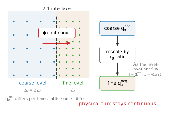
Scalar fields across a refinement interface. The concentration phi is continuous across levels, but the stored non-equilibrium flux q^neq is rescaled between levels so the physical flux stays continuous, since the lattice units differ on each side. This mirrors the fluid rule where the macroscopics are continuous but the non-equilibrium stress is rescaled.
\(q_\alpha^{neq}\) rescales between levels so that the physical scalar flux \(J^{phys}_\alpha = -D_{total}^{phys}\,\partial_\alpha \phi^{phys}\) is continuous across the interface. The Chapman-Enskog expansion of the advection-diffusion LBM gives, per level and in that level’s lattice units,
and with the 2:1 ratio (\(\Delta x_c = 2\,\Delta x_f\), \(\Delta t_c = 2\,\Delta t_f\)) the factor \(\Delta t / \Delta x\) is level-invariant, so
The implementation mirrors the fluid’s \(S \leftrightarrow \sigma\) stress conversion: the pack side converts to the level-invariant flux \(J = q^{neq}\,(\tau_g - 1/2)/\tau_g = q^{neq}\,(1 - \omega_\phi/2)\) with the source level’s relaxation, and the unpack side converts back with the target level’s relaxation.
Warning
The rescaling factor is not unity even without LES: \(\tau_g - 1/2 = D^{lbm}/c_{s,\phi}^2\) doubles per refinement level (where \(D^{lbm}(\ell) = 2^\ell D_0^{lbm}\)), so for small \(D\) the coarse \(q^{neq}\) is roughly twice the fine one. Carrying \(\phi\) across the interface unchanged while also passing \(q^{neq}\) unchanged silently corrupts the scalar flux at every refinement boundary.
When LES is active, \(D_{total}^{phys} = D_0 + \nu_{SGS}^{phys}/Sc_t\) enters \(\tau_g\) per level through the values \(\nu_{SGS,c}^{phys}\) and \(\nu_{SGS,f}^{phys}\) taken directly from the fluid interface treatment, which has already solved the Lagrava stress-matching condition; no additional non-linear solve is needed for the scalar.
Coarse-to-fine spatial interpolation reuses the existing four-point cubic scheme (three-point at borders) on \(\phi\) and component-wise on \(q_\alpha^{neq}\). Fine-to-coarse uses point injection from the coincident fine node, mirroring the fluid’s F2C treatment of \(\rho\) and \(u_\alpha\). Time interpolation at intermediate fine-time steps reuses the existing three-point Lagrange scheme. The structure mirrors the fluid F2C/C2F treatment described in Multiblock, with the simplification that the scalar flux is rank-1 and inherits \(\nu_{SGS}\) from the fluid layer.
Initialisation
The scalar follows the same three-stage initialisation as the fluid kernel:
Evaluate the user-supplied
initial_fieldsymbolic expression for \(\phi_0(x, y, z)\) and write \(\phi\) at every node.Set \(q_\alpha^{neq} = 0\) everywhere; the non-equilibrium flux builds up naturally during the first collision-streaming steps.
Run a border-collision pass that writes scalar populations on boundary nodes, analogous to the fluid border-init kernel.
All field computation happens on the GPU; CPU-side initialisation is limited to constant scalar values.
Immersed Boundary Method
Scope: solid-body scalar boundaries use voxelization
Scalar boundary conditions on solid bodies are imposed by voxelization (band-only classification of the near-surface nodes), described in Voxelization of Solid-Body Scalar Boundaries. The immersed-boundary scalar route described in this section is the diffuse-interface alternative that reuses the velocity IBM machinery. The wall reconstructions in Boundary Conditions (Dirichlet, Neumann, bounce-back) are the imposed scalar wall conditions; voxelization selects the band of nodes those conditions act on.
An immersed body in a thermal problem carries two conditions on the same Lagrangian mesh: a velocity condition on the fluid populations and a scalar condition on \(g\). The scalar IBM reuses the velocity IBM interpolation and spreading kernels Peskin[3] one-to-one, with the same Roma 2-point Dirac kernel; only the macroscopic that is corrected changes.
Key idea: one immersed-boundary machinery for velocity and scalar
The interpolation, spreading, and Dirac kernel are shared verbatim with the velocity IBM. The scalar is not a parallel implementation; it passes a different macroscopic (\(\phi\) instead of \(u_\alpha\)) through the same path. A fix to the immersed-boundary geometry handling reaches both fields at once.
The scalar boundary type is specified per geometry:
Dirichlet (\(\phi_w\) prescribed): \(\phi\) is interpolated to the Lagrangian point, and the correction needed to reach \(\phi_w\) is delivered as a scalar source whose spread increment updates the zeroth moment, \(\phi^{\text{IBM}} = \phi + \tfrac{\Delta t}{2}\,\Delta S\). As with multi-direct forcing on the velocity, a few sub-iterations on \(\Delta S\) tighten the imposed value. Only the zeroth moment is touched; the flux responds through the collision.
Neumann (\(J_w\) prescribed): the wall-normal flux is imposed by reconstruction. The scalar is sampled at an off-wall reference point a distance \(d_n\) along the normal to get \(\phi_P\), the surface value consistent with the prescribed gradient is set as \(\phi_w = \phi_P + (J_w / D_{\text{total}})\, d_n\), and that value is imposed through the Dirichlet procedure. The adiabatic case is \(J_w = 0\), i.e. \(\phi_w = \phi_P\).
Volumetric source: a distributed source (a heated solid, vegetation canopy heat exchange) is spread from the Lagrangian markers to the Eulerian \(S\) field with the same kernels, then enters the scalar collision through the source term documented in Collision and State Storage.
Invisible: the scalar ignores the body, useful for porous obstacles or geometry-only fluid IBM tests.
Bookkeeping. The scalar IBM mirrors the momentum bookkeeping: during the source/correction spread the populations \(g_i\) are held fixed, so the moments derived from them stay fixed and only \(\phi\) (and, where a flux is imposed, the first moment) is updated. After streaming, the IBM source and correction are removed and force-free scalar macroscopics are recomputed and stored, so that multiblock communication between grid levels transfers clean \((\phi, q_\alpha^{neq})\) without embedded IBM contributions.
A subtle trap: the scalar layer is thinner than the velocity layer
The thermal boundary layer scales as \(\delta_T \sim \delta / Pr^{1/3}\), so for \(Pr > 1\) it is thinner than the momentum layer. A grid that resolves the velocity near a wall may still under-resolve the scalar. Use the Dirichlet-with-reconstruction route on the reference-point normal wherever a velocity wall model is already in place, rather than assuming the scalar is resolved.
The same Dirac kernel and spreading machinery power the Lagrangian source term path documented in Collision and State Storage.