Turbulent Pipe Flow (Reynolds 180)

The simulation of a periodic turbulent pipe flow is used for the validation of the immersed boundary method effectiveness to delineate a curved boundary in a turbulent flow. As for the turbulent channel case, the external force density term represents the pressure gradient \(F_{x}=-\mathrm{d}p/\mathrm{d}x\), the regularized no-slip BC is employed at \(y=0\) and \(y=H\), and periodicity is considered in the remaining boundaries.

Note: A precursor turbulent flow is used to start the simulation and assure a turbulent flow. This field can be generated through a precursor poiseuille flow simulation with an Lagrangian body placed to generate perturbations and removed after turbulence is generated.

from nassu.cfg.model import ConfigScheme

filename = "validation/turbulence/03_turbulent_pipe_flow/03_turbulent_pipe_flow.nassu.yaml"

sim_cfgs = ConfigScheme.sim_cfgs_from_file_dct(filename)

An extra spacing of 2 lattices at each side of the cylinder is kept to assure a complete interpolation-spread procedure.

sim_cfg = next(iter(sim_cfgs.values()))

Functions used for processing of turbulent pipe

import numpy as np

import nassu.viz as common

common.use_style()

# One cached wall-normal (y) centre-line probe of the statistics export, reused
# for every macroscopic instead of rebuilding the line and re-probing per call.
_ds = sim_cfg.domain.domain_size
_line_probe = common.LineProbe.from_export(
    sim_cfg.output.exports["default_stats"].volumes["default_stats"].stats,
    sim_cfg.n_steps + 1,
    (_ds.x // 2, 0, _ds.z // 2),
    (_ds.x // 2, _ds.y - 1, _ds.z // 2),
    _ds.y,
)
# Sum 0.5 because data is cell centered in vtm
_norm_pos = (_line_probe.sample_points[:, 1] + 0.5) / (_ds.y + 1)


def get_macr_compressed(
    sim_cfg, macr_name: str, is_2nd_order: bool
) -> tuple[np.ndarray, np.ndarray]:
    name = macr_name if not is_2nd_order else f"{macr_name}_2nd"
    return _norm_pos, _line_probe.sample(name)

Results

Load values for comparison

import os

import numpy as np
import pandas as pd

comparison_folder = "validation/turbulence/03_turbulent_pipe_flow/reference"
files = ["ux_avg", "uang_rms", "ur_rms", "ux_rms"]
get_filename_csv = lambda f: os.path.join(comparison_folder, "Re_tau_180_" + f + ".csv")


df_cp = {f: pd.read_csv(get_filename_csv(f), delimiter=",") for f in files}

Friction velocity and y+ to use

# TODO(#750): verify/migrate this normalization. 0.003401361 is exactly the
# force-implied friction velocity u* = sqrt(F * R / 2) (F = 3.21368e-7, R = 72),
# but it is scaled here by a hand-tuned 0.925 factor with no documented basis.
# Re-run on GPU and decide whether the 0.925 correction is warranted; if not,
# use common.friction_velocity(sim_cfg, geometry="pipe", length=72) directly.
yp = 2.5
u_fric = 0.003401361 * 0.925

Load simulation velocity fields

pos, ux_avg = get_macr_compressed(sim_cfg, "ux", is_2nd_order=False)
pos, ux_2nd = get_macr_compressed(sim_cfg, "ux", is_2nd_order=True)
ux_rms = (ux_2nd - ux_avg**2) ** 0.5

pos, uy_avg = get_macr_compressed(sim_cfg, "uy", is_2nd_order=False)
pos, uy_2nd = get_macr_compressed(sim_cfg, "uy", is_2nd_order=True)
uy_rms = (uy_2nd - uy_avg**2) ** 0.5

pos, uz_avg = get_macr_compressed(sim_cfg, "uz", is_2nd_order=False)
pos, uz_2nd = get_macr_compressed(sim_cfg, "uz", is_2nd_order=True)
uz_rms = (uz_2nd - uz_avg**2) ** 0.5

ux_avg.shape, ux_rms.shape

((152,), (152,))

wall_pos = 5  # From 4 to 148
mid_pos = ux_avg.shape[0] // 2

ux_vals = ux_avg[wall_pos:mid_pos] / u_fric
x_vals = np.arange(len(ux_vals)) * yp

import matplotlib.pyplot as plt

fig, ax = common.fig_single()

ax.plot(
    df_cp["ux_avg"]["y+"],
    df_cp["ux_avg"]["u/u*"],
    **common.markers.exp(shape="o"),
    label="Experimental",
)
ax.plot(x_vals, ux_vals, **common.markers.sim_line(linestyle="--", linewidth=2.5), label="AeroSim")

ax.set_xscale("symlog")
ax.set_xlim((1, 170))

ax.set_ylabel("$u/u*$")
ax.set_xlabel("$y^+$")
ax.legend()

plt.tight_layout()
plt.show(fig)

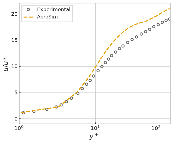
The average flow velocity shown below presents an excellent agreement with experimental results. Below, the root mean squared velocity \(u_{\alpha,\mathrm{rms}}\) is also presented against experimental data.

import matplotlib.pyplot as plt

fig, ax = common.fig_single()

get_prof_plot = lambda arr: arr[wall_pos:mid_pos] / u_fric

c_ux, c_ur, c_uang = common.colors.sim, common.colors.blue, common.colors.green

ax.plot(
    df_cp["ux_rms"]["y+"],
    df_cp["ux_rms"]["u/u*"],
    marker="o",
    fillstyle="none",
    linestyle="none",
    color=c_ux,
    markeredgewidth=1.7,
    label=r"Exp. $u_x$",
)
ax.plot(
    df_cp["ur_rms"]["y+"],
    df_cp["ur_rms"]["u/u*"],
    marker="s",
    fillstyle="none",
    linestyle="none",
    color=c_ur,
    markeredgewidth=1.7,
    label=r"Exp. $u_r$",
)
ax.plot(
    df_cp["uang_rms"]["y+"],
    df_cp["uang_rms"]["u/u*"],
    marker="D",
    fillstyle="none",
    linestyle="none",
    color=c_uang,
    markeredgewidth=1.7,
    label=r"Exp. $u_{\theta}$",
)
ax.plot(
    x_vals,
    get_prof_plot(ux_rms),
    linestyle="--",
    linewidth=1.5,
    color=c_ux,
    label=r"AeroSim $u_x$",
)
ax.plot(
    x_vals,
    get_prof_plot(uy_rms),
    linestyle="--",
    linewidth=1.5,
    color=c_ur,
    label=r"AeroSim $u_r$",
)
ax.plot(
    x_vals,
    get_prof_plot(uz_rms),
    linestyle="--",
    linewidth=1.5,
    color=c_uang,
    label=r"AeroSim $u_{\theta}$",
)

ax.legend()
ax.set_xlim((1, 170))
ax.set_xlabel("$y^+$")

plt.tight_layout()
plt.show(fig)

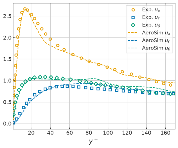
Also, an excellement agreeement is obtained for all directions in cylindrical coordinates. In general the results confirm the solver capability of solving a pipe flow turbulence, confirming the IBM as adequate to represent a curved boundary and the D3Q27 velocity set as capable of axissymetric turbulence.

Flow field

Instantaneous velocity magnitude on the pipe planes (plane_series): the longitudinal plane through the pipe axis and the cross-section at mid-length.

from nassu import viz

viz.enable_offscreen()

PANEL = (840, 320)
cfg = sim_cfgs["periodicTurbulentPipe", 0]
domain = (456.0, 152.0, 152.0)

panels = [
    viz.Panel(
        "longitudinal",
        viz.PlaneSource.from_cfg(cfg, series="plane_series", plane="longitudinal"),
        viz.frame_domain(domain, "y", panel=PANEL, slice_coord=76.0),
    ),
    viz.Panel(
        "cross-section",
        viz.PlaneSource.from_cfg(cfg, series="plane_series", plane="cross_section"),
        viz.frame_domain(domain, "x", panel=PANEL, slice_coord=228.0),
    ),
]
steps = [panels[0].source.steps[-1]]
plotter = viz.render_grid(
    panels,
    steps=steps,
    scalar="u_mag",
    cmap="viridis",
    clim=(0.0, 0.08),
    bar_title="|u|",
    panel_size=PANEL,
)
plotter.show()

/tmp/ipykernel_595898/3141045901.py:31: UserWarning: Using static image for notebook display.
Install trame for interactive backends: pip install "pyvista[jupyter]"
  plotter.show()

Version

sim_info = sim_cfg.output.read_info()

nassu_commit = sim_info["commit"]
nassu_version = sim_info["version"]
print("Version:", nassu_version)
print("Commit hash:", nassu_commit)

Version: 2.0.1a0
Commit hash: beddd3464d5add9153956c71d380b82cb4629570

Configuration

from IPython.display import Code

Code(filename=filename)

variables:
  # Wall distance from the pipe axis (centre at y=z=76, radius R=72), clamped to
  # >= 0 so the profile is finite and exactly zero at and beyond the wall. Without
  # the clamp the corners of the square domain (r > R) feed a negative argument to
  # log() and produce NaN. The envelope (1 - r^2/R^2, clamped) vanishes at the wall
  # and modulates the trip perturbations.
  wall_dist: "Max(72 - sqrt((y - 76)**2 + (z - 76)**2), 0)"
  envelope: "Max(1 - ((y - 76)**2 + (z - 76)**2)/5184, 0)"

simulations:
  - name: periodicTurbulentPipe
    save_path: ./validation/turbulence/03_turbulent_pipe_flow/results/periodic

    n_steps: 400000
    # u* = 0.0034013 / R = 72 / ETT = R/u* = 18,820
    # Re_tau = 180
    # y+ = 2.5

    report:
      frequency: 1000

    domain:
      domain_size:
        x: 456
        y: 152
        z: 152
      block_size: 8
      bodies:
        cylinder:
          geometry_path: fixture/stl/basic/cylinder.stl
          transformation:
            scale: [72, 72, 72]
            translation: [-4, 4, 4]

    data:
      exports:
        default:
          macrs: [rho, u]
          interval:
            frequency: 200000
            lvl: 0
          target:
            volume: {}
          outputs:
            instantaneous: true
        default_stats:
          macrs:
            - rho
            - u
          interval:
            frequency: 100
            start_step: 200000
            lvl: 0
          target:
            volume: {}
          outputs:
            instantaneous: false
            stats:
              macrs_1st_order:
                - rho
                - u
              macrs_2nd_order:
                - u
        plane_series:
          macrs: [rho, u]
          interval: {frequency: 40000, lvl: 0}
          target:
            planes:
              # Longitudinal plane through the pipe axis.
              longitudinal:
                axis: y
                axis_pos: 76
                dist: 1
              # Cross-section at mid-length.
              cross_section:
                axis: x
                axis_pos: 228
                dist: 1
          outputs:
            instantaneous: true

    models:
      precision:
        default: single

      LBM:
        tau: 0.504081632653061
        F:
          x: 3.21368E-07
          y: 0
          z: 0
        vel_set: D3Q27
        coll_oper: RRBGK
      initialization:
        # Reichardt mean profile (u+ = 2.5 ln(1 + 0.41 y+) + 7.8 wake), with the
        # friction velocity u* = 0.0034013 as the velocity scale and y+ = (u*/nu) d
        # = 2.5 d as the inner coordinate (nu = cs^2 (tau - 0.5) = 1.36e-3). On top
        # of it, wall-enveloped multi-mode sinusoids trip transition; the flow then
        # redevelops itself. Centreline init Ma ~ 0.13, within the Ma < 0.1 working
        # range once it relaxes.
        equations:
          rho: "1"
          ux: !sub "0.0034013*(2.5*log(1 + 0.41*2.5*${wall_dist}) + 7.8*(1 - exp(-2.5*${wall_dist}/11) - (2.5*${wall_dist}/11)*exp(-2.5*${wall_dist}/3))) + 0.010*${envelope}*cos(2*pi*4*(y - 76)/144)*cos(2*pi*3*(z - 76)/144) + 0.006*${envelope}*sin(2*pi*3*(y - 76)/144)*sin(2*pi*4*(z - 76)/144)"
          uy: !sub "0.006*${envelope}*sin(2*pi*3*x/456)*(z - 76)/72 + 0.004*${envelope}**2*cos(2*pi*2*x/456)*(z - 76)/72"
          uz: !sub "-0.006*${envelope}*sin(2*pi*3*x/456)*(y - 76)/72 - 0.004*${envelope}**2*cos(2*pi*2*x/456)*(y - 76)/72"

      engine:
        name: CUDA

      BC:
        periodic_dims: [true, false, false]
        BC_map:
          - pos: N
            BC: RegularizedHWBB
            wall_normal: N
            order: 1

          - pos: S
            BC: RegularizedHWBB
            wall_normal: S
            order: 1

          - pos: F
            BC: RegularizedHWBB
            wall_normal: F
            order: 2

          - pos: B
            BC: RegularizedHWBB
            wall_normal: B
            order: 2

      IBM:
        forces_accomodate_time: 1000
        body_cfgs:
          default: {}