
 AeroSim Docs
Flow Through Trees
The simulation of a turbulent flow through an arrangement of trees validates the solver’s volumetric quadratic (Forchheimer) canopy-drag model. Instead of resolving the canopy with an immersed-boundary point cloud, the canopy is modelled as a volumetric momentum sink applied as a fluid body force on every node inside a predicate region (models.volumetric_regions): \(F_\alpha = -\beta\,|u|\,u_\alpha\). For comparison, the results of Qi and Ishihara,
2018 and Kang et al., 2020 were used.
It consists of a 2 x 74 x 6 (m) tree arrangement positioned at 1 m height after an atmospheric flow. The drag coefficient is estimated as \(C_d = 1.6\) and the leaf area density is \(LAD = 1.16\,m^{-1}\), so the quadratic drag coefficient is derived as \(\beta_0 = 0.5\,C_d\,LAD = 0.928\) (lattice units, level 0; rescaled per level by \(1/2^{lvl}\) inside the solver). This starting value must be calibrated against the benchmark below; the domain setup is illustrated next:
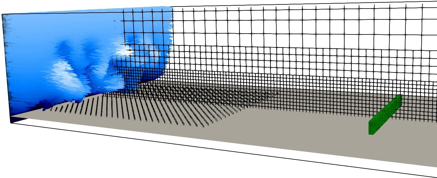
The numerical setup goal is to correctly capture both velocity and turbulent kinetic energy changes caused by the tree arrangement. The domain setup is shown below:
[1]:
from nassu.cfg.model import ConfigScheme

filename = "./validation/porous_media/01_flow_through_trees/01_flow_through_trees.nassu.yaml"

sim_cfgs = ConfigScheme.sim_cfgs_from_file_dct(filename)
[2]:
from pathlib import Path

import matplotlib.pyplot as plt
import numpy as np
import pandas as pd

import nassu.viz as common

common.use_style()

H_num = 7
scale = 1
Load experimental data:
[3]:
base_path = Path("./validation/porous_media/01_flow_through_trees/reference")
positions = ["1H", "2H", "3H", "4H", "5H"]

df_exp = []

vel = pd.read_csv(base_path / "qi2018_exp_velocity_pitot.csv")
kin = pd.read_csv(base_path / "qi2018_exp_kinetic_energy_pitot.csv")
df_csv = pd.concat([vel, kin], axis=1, join="inner")
df_exp.append(df_csv)

for pos in positions:
    vel = pd.read_csv(base_path / f"qi2018_exp_velocity_{pos}.csv")
    kin = pd.read_csv(base_path / f"qi2018_exp_kinetic_energy_{pos}.csv")
    df_csv = pd.concat([vel, kin], axis=1, join="inner")
    df_exp.append(df_csv)
[4]:
base_path = Path("./validation/porous_media/01_flow_through_trees/reference")
positions = ["1H", "2H", "3H", "4H", "5H"]

df_num2 = []

vel = pd.read_csv(base_path / "qi2018_num_velocity_pitot.csv")
kin = pd.read_csv(base_path / "qi2018_num_kinetic_energy_pitot.csv")
df_csv = pd.concat([vel, kin], axis=1, join="inner")
df_num2.append(df_csv)

for pos in positions:
    vel = pd.read_csv(base_path / f"qi2018_num_velocity_{pos}.csv")
    kin = pd.read_csv(base_path / f"qi2018_num_kinetic_energy_{pos}.csv")
    df_csv = pd.concat([vel, kin], axis=1, join="inner")
    df_num2.append(df_csv)
Results
[5]:
sim_cfg = sim_cfgs["flowThroughTrees", 0]

point_ref = sim_cfg.output.exports["velocities"].series.points["velocity_probe"].inst
df_ref = point_ref.read_full_data("ux")

df_ref = df_ref[df_ref["time_step"] > 10000]

df_point = df_ref

ux_avg = df_ref.mean()
ux_rms = df_ref.std()
Iu = ux_rms / ux_avg


u_ref = ux_avg["0"]
u_ref
[5]:
np.float32(0.023704605)
[6]:
def line_stats(position: str, u_ref) -> pd.DataFrame:
    line_ref = sim_cfg.output.exports["velocities"].series.lines[f"{position}"].inst
    df_ux = line_ref.read_full_data("ux")
    df_uy = line_ref.read_full_data("uy")
    df_uz = line_ref.read_full_data("uz")

    df_ux = df_ux[df_ux["time_step"] > 10000]
    df_uy = df_uy[df_uy["time_step"] > 10000]
    df_uz = df_uz[df_uz["time_step"] > 10000]

    ux_avg = (df_ux.mean()) / u_ref
    ux_rms = (df_ux.std()) ** 2

    uy_rms = (df_uy.std()) ** 2
    uz_rms = (df_uz.std()) ** 2

    k = (ux_rms + uy_rms + uz_rms) / (2 * u_ref**2)

    df = pd.DataFrame({"ux_avg": ux_avg, "k": k})
    df = df.drop(df.index[0])
    df["pos"] = np.linspace(0, (2 * H_num) / H_num, num=len(df), endpoint=True)
    return df
[7]:
df_num = []
df_csv = line_stats("velocity_profile", u_ref)
df_num.append(df_csv)

for pos in positions:
    df_csv = line_stats(f"pos_{pos}", u_ref)
    df_num.append(df_csv)
[8]:
def plot_curves(position: str, df_num, df_num2, df_exp):
    fig, ax = common.fig_double()
    fig.suptitle(f"{position}")

    ax[0].plot(df_num["ux_avg"], df_num["pos"], **common.markers.sim_line(), label="AeroSim")
    ax[0].plot(
        df_num2["u"],
        df_num2["z"],
        color=common.colors.blue,
        linestyle="--",
        label="Qi and Ishihara (2018)",
    )
    ax[0].plot(df_exp["u"], df_exp["z"], **common.markers.exp(shape="o"), label="Exp")
    ax[0].set_ylabel("$z/H$")
    ax[0].set_xlabel("$u/u_{H}$")
    ax[0].set_xlim(0, 2.0)
    ax[0].set_ylim(0, 1.2)
    ax[0].legend(loc="best")

    ax[1].plot(df_num["k"], df_num["pos"], **common.markers.sim_line(), label="AeroSim")
    ax[1].plot(
        df_num2["k"],
        df_num2["h"],
        color=common.colors.blue,
        linestyle="--",
        label="Qi and Ishihara (2018)",
    )
    ax[1].plot(df_exp["k"], df_exp["h"], **common.markers.exp(shape="o"), label="Exp")
    ax[1].set_ylabel("$z/H$")
    ax[1].set_xlabel("TKE/$u_{H}^{2}$")
    ax[1].set_xlim(0, 0.2)
    ax[1].set_ylim(0, 1.2)
    ax[1].legend(loc="best")

    plt.tight_layout()
    plt.show(fig)
[9]:
## Inflow plot
plot_curves("Inflow", df_num[0], df_num2[0], df_exp[0])

## Post obstacles plots
for i, pos in enumerate(positions):
    plot_curves(pos, df_num[i + 1], df_num2[i + 1], df_exp[i + 1])
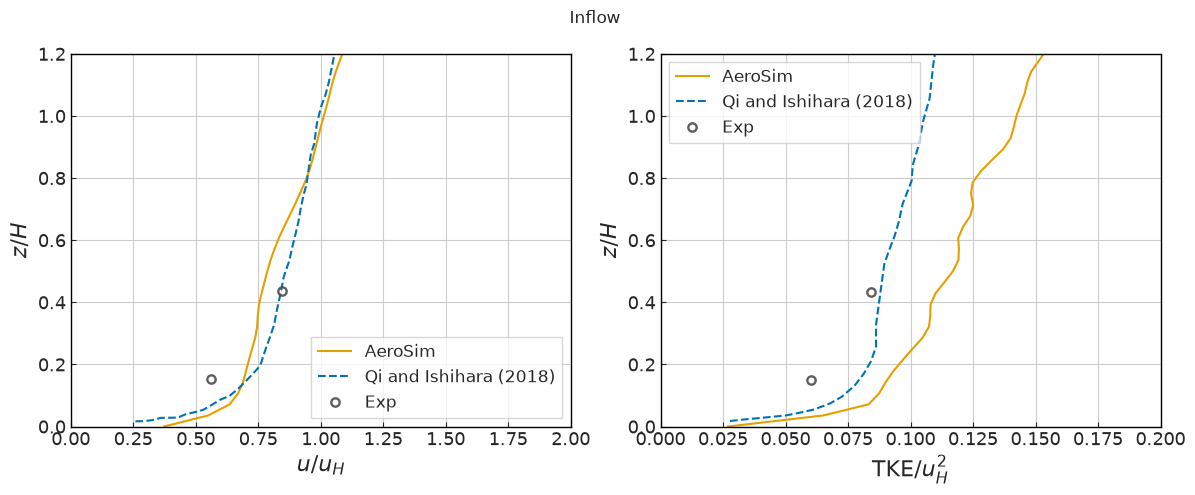
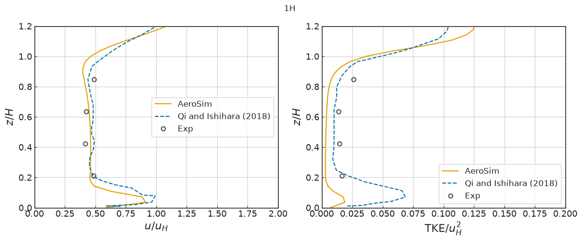
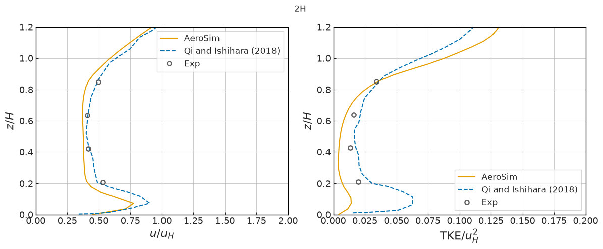
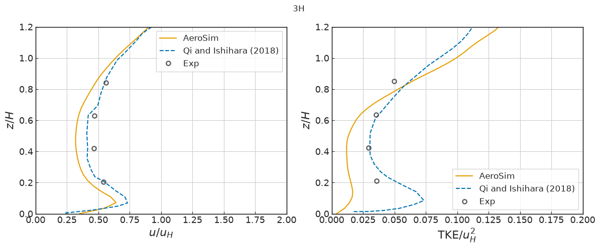
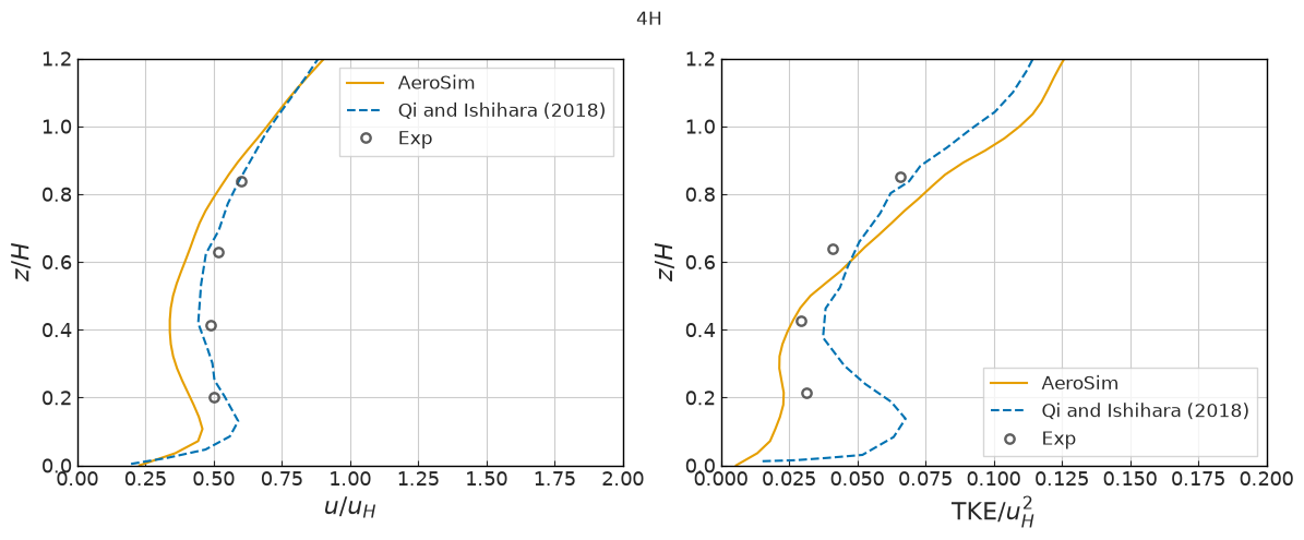
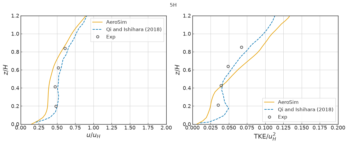
It can be seen a satisfactory match between inflow and experimental data despite the coarse resolution applied on the validation case. The qualitative aspects of the flow profile after the tree arrangement are well reproduced and quantitative aspects also have a decent representation. The difference compared to Qi and Ishihara results might be due our resolution of 0.25m against their 0.025m close to the ground.
Flow field
Instantaneous velocity magnitude on the vertical plane through the tree canopy centre (plane_series.mid_canopy).
[10]:
from nassu import viz

viz.enable_offscreen()

PANEL = (1040, 200)
cfg = sim_cfgs["flowThroughTrees", 0]
source = viz.PlaneSource.from_cfg(cfg, series="plane_series", plane="mid_canopy")
view = viz.frame_domain((600.0, 144.0, 64.0), "y", panel=PANEL, slice_coord=72.0)

steps = [source.steps[-1]]
plotter = viz.render_grid(
    [viz.Panel("mid-canopy", source, view)],
    steps=steps,
    scalar="u_mag",
    cmap="viridis",
    clim=(0.0, 0.09),
    bar_title="|u|",
    panel_size=PANEL,
)
plotter.show()
2026-07-23 02:43:04.432 (  18.443s) [    7A2020330B80]vtkXOpenGLRenderWindow.:1460  WARN| bad X server connection. DISPLAY=
/tmp/ipykernel_2104878/2872874502.py:20: UserWarning: Using static image for notebook display.
Install trame for interactive backends: pip install "pyvista[jupyter]"
  plotter.show()

Version
[11]:
sim_cfg = next(iter(sim_cfgs.values()))
sim_info = sim_cfg.output.read_info()

nassu_commit = sim_info["commit"]
nassu_version = sim_info["version"]
print("Version:", nassu_version)
print("Commit hash:", nassu_commit)
Version: 2.0.0a7
Commit hash: 5e47f2762575c2d285254d36bfd354b6af09fda1
Configuration
[12]:
from IPython.display import Code

Code(filename=filename)
[12]:
variables:
  domain:
    scale: !math 1/1
    plane_height: 4.0
    body_pos: 200
    H_ref:
    pos_025H: !math ${domain.body_pos} + 0.25*${var.H_num}
    pos_05H: !math ${domain.body_pos} + 0.5*${var.H_num}
    pos_1H: !math ${domain.body_pos} + 1.0*${var.H_num}
    pos_2H: !math ${domain.body_pos} + 2.0*${var.H_num}
    pos_3H: !math ${domain.body_pos} + 3.0*${var.H_num}
    pos_4H: !math ${domain.body_pos} + 4.0*${var.H_num}
    pos_5H: !math ${domain.body_pos} + 5.0*${var.H_num}
  var:
    H_num: !math 7*${domain.scale}

simulations:
  - name: flowThroughTrees
    save_path: ./validation/porous_media/01_flow_through_trees/results

    n_steps: 40000

    report:
      frequency: 500

    domain:
      domain_size:
        x: 600
        y: 144
        z: 64
      block_size: 8
      bodies:
        full_plane:
          IBM:
            run: true
            cfg_use: category_II
            order: 0
          geometry_path: fixture/stl/abl/ground.stl
          small_triangles: add
          transformation:
            translation: !math [0, 0, "${domain.plane_height}"]
        plates_obstacles:
          IBM:
            order: 1
          geometry_path: fixture/stl/abl/roughness_elements_cat2.stl
          volumes_limits:
            body_transformed:
              - start: !math [10, 20, 0]
                end: !math [120, 124, 64]
          small_triangles: add
          transformation:
            translation: !math [0, 1, "${domain.plane_height}"]
            scale: !math [1.25, 1.25, "20.0*${domain.scale}"] #2m

      refinement:
        static:
          default:
            volumes_refine:
              # - start: [0, 56, 2]
              #   end: [256, 88, 12]
              #   lvl: 3
              #   is_abs: true
              - start: [0, 34, 0]
                end: [288, 110, 24]
                lvl: 2
                is_abs: true
              - start: [0, 0, 0]
                end: [352, 144, 40]
                lvl: 1
                is_abs: true

    data:
      monitors:
        fields:
          rho_max:
            macrs: [rho]
            stats: [min, max]
            interval: {start_step: 500, frequency: 50}
      exports:
        full_domain:
          macrs: [rho, u, omega_LES, f_IBM]
          interval:
            frequency: 10000
            lvl: 0
          target:
            volumes:
              full_domain: {}
          outputs:
            instantaneous: true
        full_domain_stats:
          macrs:
            - rho
            - u
          interval:
            frequency: 10
            start_step: 10000
            lvl: 0
          target:
            volumes:
              full_domain_stats: {}
          outputs:
            instantaneous: false
            stats:
              macrs_1st_order:
                - rho
                - u
              macrs_2nd_order:
                - u
        velocities:
          macrs: ["u"]
          interval: {frequency: 10, lvl: 0}
          target:
            lines:
              inlet_profile:
                dist: 0.25
                start: !math [0, 72.0, "${domain.plane_height}"]
                end: !math [0, 72.0, "${domain.plane_height} + 14*${domain.scale}"]
              velocity_profile:
                dist: 0.25
                start: !math ["${domain.body_pos}-50*${domain.scale}", 72.0, "${domain.plane_height}"]
                end: !math ["${domain.body_pos}-50*${domain.scale}", 72.0, "${domain.plane_height} + 14*${domain.scale}"]
              pos_025H:
                dist: 0.25
                start: !math ["${domain.pos_025H}", 72.0, "${domain.plane_height}"]
                end: !math ["${domain.pos_025H}", 72.0, "${domain.plane_height} + 14*${domain.scale}"]
              pos_05H:
                dist: 0.25
                start: !math ["${domain.pos_05H}", 72.0, "${domain.plane_height}"]
                end: !math ["${domain.pos_05H}", 72.0, "${domain.plane_height} + 14*${domain.scale}"]
              pos_1H:
                dist: 0.25
                start: !math ["${domain.pos_1H}", 72.0, "${domain.plane_height}"]
                end: !math ["${domain.pos_1H}", 72.0, "${domain.plane_height} + 14*${domain.scale}"]
              pos_2H:
                dist: 0.25
                start: !math ["${domain.pos_2H}", 72.0, "${domain.plane_height}"]
                end: !math ["${domain.pos_2H}", 72.0, "${domain.plane_height} + 14*${domain.scale}"]
              pos_3H:
                dist: 0.25
                start: !math ["${domain.pos_3H}", 72.0, "${domain.plane_height}"]
                end: !math ["${domain.pos_3H}", 72.0, "${domain.plane_height} + 14*${domain.scale}"]
              pos_4H:
                dist: 0.25
                start: !math ["${domain.pos_4H}", 72.0, "${domain.plane_height}"]
                end: !math ["${domain.pos_4H}", 72.0, "${domain.plane_height} + 14*${domain.scale}"]
              pos_5H:
                dist: 0.25
                start: !math ["${domain.pos_5H}", 72.0, "${domain.plane_height}"]
                end: !math ["${domain.pos_5H}", 72.0, "${domain.plane_height} + 14*${domain.scale}"]
            points:
              velocity_probe:
                pos: !math ["${domain.body_pos}-50*${domain.scale}", 72, "${domain.plane_height} + 7*${domain.scale}"]
          outputs:
            instantaneous: true
        plane_series:
          macrs: ["u"]
          interval: {frequency: 5000, lvl: 0}
          target:
            planes:
              # Coarse vertical overview plane through the canopy centre
              # (one node apart, full domain): debug-grade view.
              mid_canopy:
                axis: y
                axis_pos: 72
                dist: 1
          outputs:
            instantaneous: true
        plane_series_roi:
          macrs: ["u"]
          interval: {frequency: 2000, lvl: 0}
          target:
            planes:
              # Fine plane restricted to the canopy region of interest
              # (canopy at x = 200, H = 7).
              mid_canopy_roi:
                axis: y
                axis_pos: 72
                min: !math ["${domain.body_pos} - 8*${var.H_num}", 0]
                max: !math ["${domain.body_pos} + 12*${var.H_num}", "4*${var.H_num}"]
                dist: 0.25

          outputs:
            instantaneous: true
    models:
      precision:
        default: single

      LBM:
        tau: 0.500011
        vel_set: D3Q27
        coll_oper: RRBGK
      initialization:
        inlet_field: true

      engine:
        name: CUDA

      BC:
        periodic_dims: [false, false, false]
        BC_map:
          - pos: E
            BC: RegularizedNeumannOutlet
            wall_normal: E
            order: 2

            params:
              rho: 1.0
          - pos: F
            BC: Neumann
            wall_normal: F
            order: 1

          - pos: B
            BC: RegularizedHWBB
            wall_normal: B
            order: 1

          - pos: N
            BC: Neumann
            wall_normal: N
            order: 0

          - pos: S
            BC: Neumann
            wall_normal: S
            order: 0
        inlet_turbulence:
          type: sem
          eddies:
            lengthscale: {x: 20, y: 20, z: 20}
            domain_limits_yz:
              start: [20, -20]
              end: [124, 40]
          profile:
            csv_profile_data: "fixture/SEM/category_vprofile/profile_log_cat4_H150_Uh0.06.csv"
            z_offset: !math "${domain.plane_height}"
            K: 1.0

      LES:
        model: Smagorinsky
        sgs_cte: 0.17

      # Canopy quadratic (Forchheimer) drag region: F = -beta * |u| * u, applied
      # as a fluid Guo body force over the canopy bounding box. Migrated from the
      # IBM point-cloud canopy (kinetic_energy_correction) per #743. The bbox is
      # the transformed extent of fixture/point_clouds/cube_2x74x6.csv
      # (scale [1,1,1], translation [200, 72, 5.0=1.0+plane_height]).
      # beta starting value derived from the canopy Cd*LAD (0.5 * Cd * LAD =
      # 0.5 * 1.6 * 1.16 = 0.928); PENDING GPU calibration against the
      # Qi & Ishihara (2018) benchmark - not yet validated.
      volumetric_regions:
        - pos: "(x >= 200) & (x <= 202) & (y >= 35) & (y <= 109) & (z >= 5) & (z <= 11)"
          porous_alpha: 0.0
          porous_beta: !math 0.5*1.6*1.16

      IBM:
        body_cfgs:
          category_II:
            n_iterations: 3
            forces_factor: 0.5
            wall_model:
              name: EqLog
              dist_ref: 3.125
              dist_shell: 0.125
              start_step: 5000
              params:
                z0: !math "0.01*${domain.scale}"
                TDMA_max_error: 1e-04
                TDMA_max_iters: 10
                TDMA_min_div: 51
                TDMA_max_div: 51
          default: {}