The thermally-stratified atmospheric boundary layer

The turbulent-inflow chapter treats the atmospheric boundary layer (ABL) as mechanically neutral: the mean wind is the logarithmic profile set by friction and roughness, and the turbulence is whatever the SEM or a precursor supplies. That picture holds only when the ground and the air are at the same temperature. On a sunny day the ground is warmer than the air above it and buoyancy adds turbulence; on a clear night the ground is colder and buoyancy suppresses it. This page restores that thermodynamic degree of freedom to the ABL, through the thermal route already established in the thermodynamics chapter: a buoyancy-carrying active scalar coupled back to momentum by a single Boussinesq body force. It underpins the stratified-ABL and urban pollutant-dispersion validation cases.

1. Motivation and stratification regimes

Wind loads, pedestrian comfort and, above all, pollutant dispersion in cities are set by the turbulence in the lowest tens of metres of the atmosphere, and that turbulence is not governed by shear alone. Whenever the ground and the near-surface air differ in temperature, a vertical density gradient develops and gravity does work on vertical motions. This buoyant production of turbulent kinetic energy (TKE) adds to, or subtracts from, the shear production, and its sign fixes the regime Turner[1]:

• Unstable (convective) stratification. The surface is warmer than the air, so a parcel displaced upward is lighter than its surroundings and keeps rising: buoyancy produces TKE, thickens the mixed layer and intensifies vertical exchange. This is the daytime regime, and the one both benchmarks below target Jiang and Yoshie[2], Zhou et al.[3].

• Neutral stratification. Surface and air temperatures match, buoyancy neither produces nor destroys TKE, and the ABL reduces to the purely mechanical logarithmic layer of the inflow chapter.

• Stable stratification. The surface is colder than the air, so a displaced parcel is heavier than its surroundings and sinks back: buoyancy consumes TKE, damps vertical motion and can laminarise the near-surface flow. This is the night-time regime, the hardest to reproduce and the one most associated with pollutant trapping.

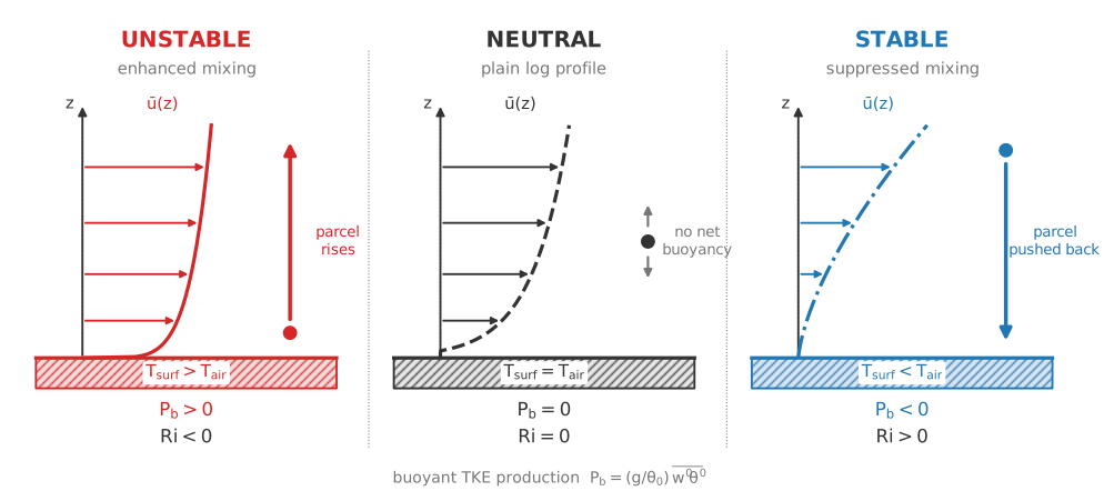
The sign of near-surface buoyancy selects the stratification regime: a warm floor (unstable) produces TKE and mixes momentum into a fuller, less-sheared wind profile, equal temperatures (neutral) leave the plain logarithmic profile, and a cold floor (stable) consumes TKE and leaves a more strongly sheared profile, matching the sign of the buoyant production \(P_b\) and of the gradient Richardson number.

Two numbers name the regime

The gradient Richardson number compares the buoyant destruction of TKE to its shear production, using local gradients,

(1)\[ \mathrm{Ri} = \frac{\dfrac{g}{\theta_0}\,\dfrac{\partial \bar\theta}{\partial z}} {\left(\dfrac{\partial \bar u}{\partial z}\right)^{2}}, \]

with \(\theta_0\) a reference (potential) temperature and \(g\) the gravitational acceleration. \(\mathrm{Ri} < 0\) is unstable, \(\mathrm{Ri} = 0\) neutral, \(\mathrm{Ri} > 0\) stable. Because \(\partial\bar u/\partial z\) and \(\partial\bar\theta/\partial z\) are awkward to evaluate at a wall, wind-tunnel and CFD studies more often report a bulk Richardson number built from finite differences across a reference height. The two benchmarks below each define their own, so bulk-Richardson values are not directly comparable between studies.

The Monin-Obukhov framing of Section 2 makes the same statement with a length rather than a ratio: the Obukhov length \(L\) is the height at which buoyant and shear production become comparable, so \(z/L\) plays the role of \(\mathrm{Ri}\) through the surface layer. The classical Pasquill-Gifford stability classes A-F used in regulatory Gaussian-plume dispersion Turner[1] are a coarse binning of exactly this axis, from strongly convective (A) through neutral (D) to strongly stable (F).

2. Monin-Obukhov similarity theory

Monin-Obukhov similarity theory (MOST) extends the neutral law of the wall (derived here) to a stratified surface layer. The neutral argument had a single velocity scale \(u^{*}\) and a single length \(z\); MOST adds a second length, the Obukhov length

(2)\[ L = -\,\frac{u^{*3}\,\theta_0}{\kappa\, g\, \overline{w'\theta'}_0}, \]

where \(\overline{w'\theta'}_0\) is the surface kinematic heat flux, \(\kappa \approx 0.41\) the von Karman constant and \(\theta_0\) a reference potential temperature. An upward (warming) surface flux \(\overline{w'\theta'}_0 > 0\) makes the length negative, \(L < 0\), which is the unstable regime; \(L > 0\) is stable and \(|L| \to \infty\) is neutral. The dimensionless stability parameter is \(\zeta = z/L\). This sign convention is used consistently throughout the page.

Nassu carries the buoyancy through the Boussinesq scalar of Section 3, where the buoyant forcing per unit scalar is \(\beta\,g\) rather than \(g/\theta_0\). The wall model therefore uses the buoyancy strength \(B \equiv \beta\,|\mathbf g|\) read from the coupling scalar’s Boussinesq block in place of \(g/\theta_0\), so (2) becomes \(L = -u^{*3}/(\kappa\,B\,\overline{w'\theta'}_0)\). Sharing \(\beta g\) with the fluid body force guarantees the wall model and the resolved buoyancy cannot disagree on the stratification strength.

Dimensional analysis then fixes the stability-corrected gradients. The mean-wind and mean-temperature gradients become

(3)\[ \frac{\partial \bar u}{\partial z} = \frac{u^{*}}{\kappa z}\,\phi_m\!\left(\zeta\right), \qquad \frac{\partial \bar\theta}{\partial z} = \frac{\theta^{*}}{\kappa z}\,\phi_h\!\left(\zeta\right), \qquad \theta^{*} \equiv -\,\frac{\overline{w'\theta'}_0}{u^{*}}, \]

with \(\phi_m, \phi_h\) the universal stability functions and \(\theta^{*}\) the temperature scale. Integrating from the roughness length \(z_0\) upward gives the stability-corrected log law that generalises the neutral profile,

(4)\[ \bar u(z) = \frac{u^{*}}{\kappa}\left[\ln\!\left(\frac{z}{z_0}\right) - \psi_m\!\left(\frac{z}{L}\right)\right], \qquad \bar\theta(z) - \theta_s = \frac{\theta^{*}}{\kappa}\left[\ln\!\left(\frac{z}{z_{0h}}\right) - \psi_h\!\left(\frac{z}{L}\right)\right], \]

where \(\theta_s\) is the aerodynamic surface temperature, \(z_{0h}\) the roughness length for heat, and \(\psi_m, \psi_h\) the integrated stability corrections, \(\psi(\zeta) = \int_0^{\zeta}[1-\phi(\zeta')]\,\mathrm{d}\zeta'/\zeta'\). The heat roughness \(z_{0h}\) is generally smaller than the momentum \(z_0\); their ratio is an empirical input that a validation case must fix from a cited source rather than assume equal. Setting \(\psi_m = \psi_h = 0\) recovers the neutral profile of the inflow chapter exactly, so the stratified law is a strict extension of the neutral one.

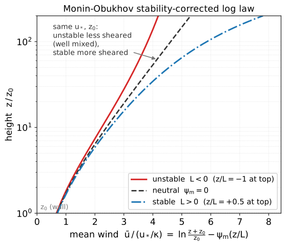
Stability-corrected log-law mean-wind profiles for one \(u_*\) and \(z_0\): the unstable (convective) profile is less sheared and well mixed, the stable (night-time) profile more sheared, and neutral recovers the plain log law when \(\psi_m = 0\). This is the profile ordering Nassu’s GPU differential test reproduces.

The universal functions are empirical. The widely used Businger-Dyer / Paulson forms are, for the unstable branch (\(\zeta < 0\)), with \(x = (1 - \gamma\,\zeta)^{1/4}\),

(5)\[ \psi_m(\zeta) = 2\ln\!\frac{1+x}{2} + \ln\!\frac{1+x^{2}}{2} - 2\arctan x + \frac{\pi}{2}, \qquad \psi_h(\zeta) = 2\ln\!\frac{1+x^{2}}{2}, \]

and for the stable branch (\(\zeta > 0\)) the linear form \(\psi_m(\zeta) = \psi_h(\zeta) = -\beta_s\,\zeta\). The coefficients \(\gamma\) and \(\beta_s\) are empirical and source-dependent (commonly \(\gamma \approx 16\), \(\beta_s \approx 5\), but \(\gamma = 15\) and \(\beta_s = 4.7\) are also in use), so each validation case must cite the specific values it adopts.

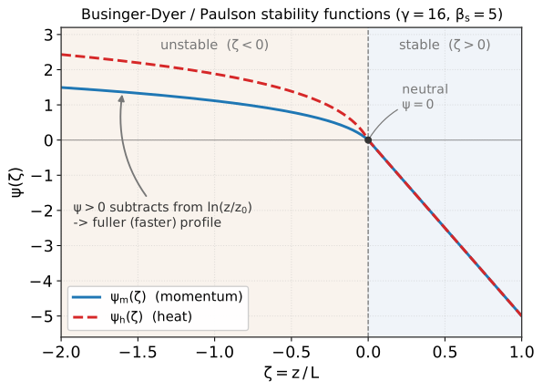
The integrated stability corrections \(\psi_m\) (momentum) and \(\psi_h\) (heat): both vanish at neutral (\(\zeta = 0\)), rise positive on the unstable side where they subtract from \(\ln(z/z_0)\) to fill out the mean profile, and fall along the common linear branch \(-\beta_s\,\zeta\) on the stable side. Curves are evaluated from the same nassu.IBM.mo_stability code the wall model uses.

The surface-layer relation between the local \(\mathrm{Ri}\) of (1) and \(\zeta = z/L\) follows from (3), \(\mathrm{Ri} = \zeta\,\phi_h(\zeta)/\phi_m^{2}(\zeta)\), so \(\mathrm{Ri} \to \zeta\) in the neutral limit. This is the tie between the two framings of Section 1.

Why this grounds the IBM wall-model correction

Equation (4) is the stratified generalisation of the log law the IBM wall model imposes at building and ground surfaces. Under stratification the friction velocity recovered from the matching-point tangential velocity acquires the \(\psi_m(z/L)\) correction. Nassu drives this flux-driven: the surface kinematic heat flux \(\overline{w'\theta'}_0\) is prescribed directly and forms \(L\) through (2), so no surface-temperature or temperature-scale inversion is needed and the momentum wall model never samples the scalar field. Because \(u^{*}\) and \(L\) are coupled through (2) and (4), they are converged together by a short fixed-point (Picard) iteration seeded from the neutral \(u^{*}\). The argument \(\zeta = z/L\) is clamped to the surface-layer validity range: besides respecting MOST validity this breaks the positive feedback of the stable-branch \(u^{*}\) iteration, which would otherwise drive \(u^{*}\to 0\), \(L\to 0\) and \(\zeta\to\infty\).

Implementation status

The Monin-Obukhov correction of this section and the height-varying (stratified) scalar inlet are implemented in epic #1034 P4 (the IBM EqLog wall model applies the \(\psi_m(z/L)\)-corrected log law, and equation-form scalar inlet / wall values are baked per node into the scalar BC kernels). The correction is flux-driven (fix #1043): the surface kinematic heat flux is prescribed directly through surface_heat_flux and \(u^{*}\) and \(L\) are converged by a short Picard iteration. The stability-function coefficients are hard-coded to \(\gamma = 16\), \(\beta_s = 5\); as noted above, a validation case must cite the coefficients it adopts. The wall model has been GPU-validated by a differential neutral / unstable / stable sign check (epic #1034 P5).

3. Boussinesq scalar buoyancy in the LBM

Nassu carries stratification through the constant-density Boussinesq route of the modeling hierarchy. A single active scalar \(b\) - a buoyancy variable proportional to the potential-temperature perturbation, \(b \equiv \bar\theta - \theta_{\text{ref}}\) - is transported on the existing double-distribution scalar path, obeying the plain advection-diffusion equation

(6)\[ \partial_t b + u_\alpha \partial_\alpha b = D\,\nabla^2 b + S_b, \]

with \(D\) the diffusivity (molecular plus the subgrid contribution when LES is active) and \(S_b\) any surface or volumetric source. The scalar is active, not passive, because it feeds back to the momentum equation through one term only, the Boussinesq body force

(7)\[ F^{\text{buoy}}_\alpha = \rho_0\,\beta\,b\,g\,\hat e_z, \]

with \(\beta\) the thermal expansion coefficient, \(\rho_0\) the constant reference density and \(\hat e_z\) the vertical unit vector, so a warm parcel (\(b>0\)) is pushed upward.

The force (7) enters the fluid not by modifying the equilibrium but through the Guo forcing scheme as the body-force density \(g_\alpha\). It contributes the half-step velocity correction \(\rho u_\alpha = \sum_i f_i c_{i,\alpha} + \tfrac{\Delta t}{2} F^{\text{buoy}}_\alpha\) and the Guo source populations documented on the lattice-unit page. The fluid collision operator itself is untouched: the coupling is one additive force term, evaluated from the current scalar field each step.

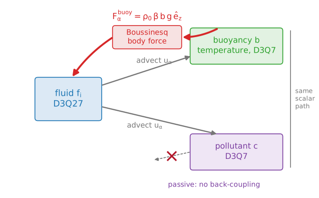
The fluid velocity advects both scalars on one shared double-distribution path, but only the active buoyancy scalar \(b\) feeds back to momentum, through the single Boussinesq body force; the pollutant is passive with no back-coupling.

Why the scalar-Boussinesq route, not an energy equation or the EOS

Three thermal routes exist in the hierarchy; the ABL uses the weakest deliberately.

• The perturbations are small. A daytime near-surface air-ground difference of a few to a few tens of kelvin gives \(\beta\,\Delta T \sim 10^{-2}\) to \(10^{-1}\), well inside the Boussinesq small-\(\Delta T\) envelope \(\beta\,\Delta T \ll 1\). Reproducing the density field to fire-scale accuracy is unnecessary; reproducing the buoyant forcing is the whole physics, and that is exactly what (7) supplies.

• It is more numerically stable. The Boussinesq route keeps the fluid zeroth moment as the density and touches the collision only through an additive force. The variable-density low-Mach closure instead reinterprets the zeroth moment as reduced pressure and slaves density to temperature through the equation of state, which admits the checkerboard pressure mode analysed on the stability page. The ABL does not need that machinery.

• It reuses one code path. \(b\) rides the same scalar transport, multiblock flux rescaling and LES subgrid closure (\(D_{\text{SGS}} = \nu_{\text{SGS}}/Sc_t\)) as any tracer. There is no energy solver and no equation of state to maintain.

Surface boundaries: IBM for momentum, voxelization for the scalar

The building and ground momentum boundaries are imposed by the immersed boundary method (optionally with the stratified wall-model correction of Section 2), while the surface heat/scalar condition on \(b\) - a prescribed wall value or a prescribed wall-normal flux - is imposed by voxelization on the near-surface band rather than by an equilibrium wall-model BC. A prescribed surface heat flux is the natural driver here, because it sets \(\overline{w'\theta'}_0\) and therefore the Obukhov length (2) directly.

The mean part of the inflow is the stratified profile (4), and the fluctuations come from the SEM or a precursor as in the neutral case; the scalar carries a matching mean temperature profile and, where available, its own fluctuation statistics. As the inflow chapter stresses, the inlet and the ground are one boundary condition: under stratification they must agree not only on \(z_0\) but on the surface heat flux, or the boundary layer re-equilibrates over the fetch.

4. Dispersion in the stratified ABL

Pollutant transport rides the same scalar machinery: a passive tracer \(c\) obeys (6) with its own source, decoupled from momentum (no buoyancy force). Field studies and wind-tunnel benchmarks report the normalised concentration

(8)\[ K \equiv \frac{\langle c\rangle\, U_H\, H^{2}}{q} = \frac{\langle c\rangle}{C_0}, \qquad C_0 = \frac{q}{U_H H^{2}}, \]

with \(q\) the volumetric emission rate, \(U_H\) the reference velocity at building height \(H\), and \(C_0\) the reference concentration; this is the normalisation both benchmarks use Jiang and Yoshie[2], Zhou et al.[3]. The mechanism by which stratification changes dispersion is read most cleanly from the flux decomposition of the mean scalar transport across a surface,

(9)\[ Q_\alpha = \underbrace{\langle u_\alpha\rangle\langle c\rangle}_{\text{advection } Q_{a}} + \underbrace{\langle u_\alpha' c'\rangle}_{\text{turbulent } Q_{t}} - \underbrace{D\,\partial_\alpha\langle c\rangle}_{\text{molecular } Q_{m}}, \]

as used by Jiang and Yoshie[2], Zhou et al.[3] and Bazdidi-Tehrani et al.[4]. Three robust, benchmark-supported effects of increasing instability follow.

• Enhanced vertical mixing lowers near-ground concentration. Buoyant TKE production raises the vertical turbulent flux \(Q_t\), venting the tracer out of street canyons and wakes and reducing \(K\) near the source. Jiang and Yoshie[2] show for a 3-D street canyon that the roof-level exchange is turbulence-dominated.

• Wakes and recirculation shrink. Zhou et al.[3] report that for an isolated rectangular building the streamwise length of the leeward recirculation region shrinks by \(32\%\) as \(\mathrm{Ri}\) goes from \(0\) to \(-1.5\), and that inside that region the advection flux \(Q_a\) reaches roughly four times the turbulent-diffusion flux \(Q_t\) at \(\mathrm{Ri} = -1.5\). The mean flow, not turbulent diffusion, therefore controls transport in the near wake even as instability grows.

• Turbulent transport can run counter to the mean gradient. Bazdidi-Tehrani et al.[4], decomposing the convective and turbulent diffusion fluxes around a high-rise building across the stable, neutral and unstable regimes, show that LES reproduces the counter-gradient mechanism - a turbulent flux directed up the mean concentration gradient - which the gradient-diffusion closures of RANS cannot represent. This is a further reason the buoyancy-driven dispersion cases here are run with LES rather than RANS.

Where this sits in the CFD-dispersion landscape

Urban pollutant dispersion is now routinely tackled with CFD, but the systematic review of Pantusheva et al.[5] finds that many published studies omit model-setup details needed to reproduce them and that few carry out formal verification and validation. LES outperforms RANS for the unsteady, buoyancy-driven transport of these flows, but it is far more sensitive to the inflow turbulence: the tracer field responds directly to the resolved eddies, so a poorly conditioned inlet corrupts the concentration field even when the mean wind is correct Ghane-Tehrani and Ziaei-Rad[6] - an effect first shown for a non-isothermal high-rise building by Yoshie et al.[7], whose LES matched the wind-tunnel gas dispersion only once inflow turbulence was supplied. That sensitivity, together with the need for a divergence-free stratified inlet, is why the ABL-dispersion cases lean on the well-conditioned synthetic and spectral inflow generators - digital-filter Klein et al.[8], divergence-free synthetic-eddy Poletto et al.[9], Kim et al.[10], spectral Melaku and Bitsuamlak[11] and optimised-ABL Lamberti et al.[12] methods - reviewed in the inflow chapter, and validate against the stratified wind-tunnel benchmarks of Jiang and Yoshie[2] and Zhou et al.[3] (see also the accidental-release review Dou and others[13]).

---

[1] (1,2)

D. Bruce Turner. Workbook of Atmospheric Dispersion Estimates: An Introduction to Dispersion Modeling. CRC Press, 2 edition, 1994. ISBN 978-1-56670-023-8.

[2] (1,2,3,4,5)

Guangyu Jiang and Ryuichiro Yoshie. Large-eddy simulation of flow and pollutant dispersion in a 3D urban street model located in an unstable boundary layer. Building and Environment, 142:47–57, 2018. doi:10.1016/j.buildenv.2018.06.015.

[3] (1,2,3,4,5)

Xing Zhou, Aotian Ying, Beihua Cong, Hideki Kikumoto, Ryozo Ooka, Liang Kang, and Hongyuan Hu. Large eddy simulation of the effect of unstable thermal stratification on airflow and pollutant dispersion around a rectangular building. Journal of Wind Engineering and Industrial Aerodynamics, 211:104526, 2021. doi:10.1016/j.jweia.2021.104526.

[4] (1,2)

Farzad Bazdidi-Tehrani, Payam Gholamalipour, Mohsen Kiamansouri, and Mohammad Jadidi. Large eddy simulation of thermal stratification effect on convective and turbulent diffusion fluxes concerning gaseous pollutant dispersion around a high-rise model building. Journal of Building Performance Simulation, 12(1):97–116, 2019. doi:10.1080/19401493.2018.1486886.

[5]

Mariya Pantusheva, Radostin Mitkov, Petar O. Hristov, and Dessislava Petrova-Antonova. Air pollution dispersion modelling in urban environment using CFD: a systematic review. Atmosphere, 13(10):1640, 2022. doi:10.3390/atmos13101640.

[6]

Elham Ghane-Tehrani and Masoud Ziaei-Rad. A comparative study of synthetic turbulence inflow approaches for air pollution simulation. Environmental Modelling & Software, 193:106639, 2025. doi:10.1016/j.envsoft.2025.106639.

[7]

Ryuichiro Yoshie, Guoyi Jiang, Taichi Shirasawa, and Jaeyong Chung. CFD simulations of gas dispersion around high-rise building in non-isothermal boundary layer. Journal of Wind Engineering and Industrial Aerodynamics, 99:279–288, 2011. doi:10.1016/j.jweia.2011.01.006.

[8]

M. Klein, A. Sadiki, and J. Janicka. A digital filter based generation of inflow data for spatially developing direct numerical or large eddy simulations. Journal of Computational Physics, 186(2):652–665, 2003.

[9]

Ruggero Poletto, Tim Craft, and Alistair Revell. A new divergence free synthetic eddy method for the reproduction of inlet flow conditions for LES. Flow, Turbulence and Combustion, 91(3):519–539, 2013. doi:10.1007/s10494-013-9488-2.

[10]

Yusik Kim, Ian P. Castro, and Zheng-Tong Xie. Divergence-free turbulence inflow conditions for large-eddy simulations with incompressible flow solvers. Computers & Fluids, 84:56–68, 2013. doi:10.1016/j.compfluid.2013.06.001.

[11]

Abiy F. Melaku and Girma T. Bitsuamlak. A divergence-free inflow turbulence generator using spectral representation method for large-eddy simulation of abl flows. Journal of Wind Engineering and Industrial Aerodynamics, 212:104580, 2021. doi:10.1016/j.jweia.2021.104580.

[12]

Giacomo Lamberti, Clara García-Sánchez, Jorge Sousa, and Catherine Gorlé. Optimizing turbulent inflow conditions for large-eddy simulations of the atmospheric boundary layer. Journal of Wind Engineering and Industrial Aerodynamics, 177:32–44, 2018. doi:10.1016/j.jweia.2018.04.004.

[13]

Zhan Dou and others. Atmospheric dispersion prediction of accidental release: a review. Emergency Management Science and Technology, 2:9, 2022. doi:10.48130/EMST-2022-0009.