Passive Scalar Diffusion - Spatial Convergence (Case 12a)

This notebook validates the scalar advection-diffusion (DDF) module against the exact analytical solution for a single Fourier mode diffusing on a periodic 3-D box. With the fluid stationary the advection term vanishes, isolating the scalar collision-streaming kernel.

The initial scalar field on a periodic domain \([0, N)^3\) is:

\[\phi(x, y, z, 0) = \cos(k x), \quad k = 2\pi / N\]

A single Fourier mode is an eigenfunction of the Laplacian, so the analytical solution is an exact exponential decay valid for all \(t > 0\):

\[\phi(x, y, z, t) = \cos(k x) \, e^{-D k^2 t}\]

Protocol: \(D = 0.05\) in lattice units, constant across all grids. Each simulation runs for \(n_{\text{steps}} = 1 / (D k^2) = N^2 / (D \cdot 4\pi^2)\) steps, so the analytical decay reaches one e-folding (\(e^{-1} \approx 0.368\)) at the final step.

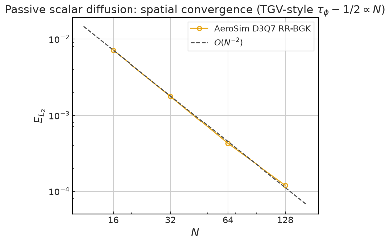
Four grids (\(N = 16, 32, 64, 128\)) are compared. The \(L_2\) error in \(\phi\) should decrease as \(O(\Delta x^2)\) on a log-log plot.

Setup

import matplotlib.pyplot as plt
import numpy as np

import nassu.viz as common
from nassu.cfg.model import ConfigScheme

common.use_style()

Load simulation configuration

filename = "validation/scalar_transport/01_passive_scalar_transport/01_passive_scalar_transport.nassu.yaml"
sim_cfgs = ConfigScheme.sim_cfgs_from_file_dct(filename)

# Unrolled simulations: sim_id 0..3 correspond to N = 16, 32, 64, 128.
sim_cfgs_list = [sim_cfgs["passiveScalarDiffusion3D", i] for i in range(4)]

# Protocol constants (in lattice units).
PHI_AMPLITUDE = 1.0

# Derive per-grid quantities from the unrolled configs. With the TGV-style
# scaling tau-0.5 ~ N, the scalar diffusivity D varies with grid size, so
# we keep a per-N dict instead of a single scalar.
GRID_SIZES = [sim_cfg.domain.domain_size.x for sim_cfg in sim_cfgs_list]
N_STEPS = {cfg.domain.domain_size.x: cfg.n_steps for cfg in sim_cfgs_list}
D_LBM = {
    cfg.domain.domain_size.x: cfg.models.scalar_transports["scalar"].adv_diff_equation.D
    for cfg in sim_cfgs_list
}

for N in GRID_SIZES:
    D = D_LBM[N]
    k = 2.0 * np.pi / N
    decay_rate = D * k**2
    decay_at_end = np.exp(-decay_rate * N_STEPS[N])
    print(
        f"N={N:3d}: D={D:.5f}, k={k:.4f}, decay_rate={decay_rate:.6f}, "
        f"steps={N_STEPS[N]}, exp(-D k^2 t_end)={decay_at_end:.4f}"
    )

N= 16: D=0.00025, k=0.3927, decay_rate=0.000039, steps=1280, exp(-D k^2 t_end)=0.9518
N= 32: D=0.00050, k=0.1963, decay_rate=0.000019, steps=2560, exp(-D k^2 t_end)=0.9518
N= 64: D=0.00100, k=0.0982, decay_rate=0.000010, steps=5120, exp(-D k^2 t_end)=0.9518
N=128: D=0.00200, k=0.0491, decay_rate=0.000005, steps=10240, exp(-D k^2 t_end)=0.9518

Analytical solution

The exact scalar field at any time \(t\) is the IC modulated by the exponential decay \(e^{-D k^2 t}\). The shape never changes - only the amplitude.

def analytical_phi(N, D, n_steps):
    """Exact scalar field at step `n_steps` on integer lattice positions.

    Convention matches the YAML initial_field: phi(x, t) = cos(2*pi*x/N) * exp(-D k^2 t).
    Returns a (N, N, N) array with axis order (x, y, z).
    """
    k = 2.0 * np.pi / N
    x = np.arange(N)
    decay = np.exp(-D_LBM[N] * k**2 * n_steps)
    profile_x = np.cos(k * x) * decay
    # Broadcast along y and z (the IC is constant in y and z, so the analytical
    # solution is too).
    return np.broadcast_to(profile_x[:, None, None], (N, N, N)).copy()


def l2_phi_error(phi_lbm, phi_exact, amplitude):
    """Normalised L2 phi error.

    E_L2 = (1/phi_amplitude) * sqrt( mean( (phi_lbm - phi_exact)^2 ) )
    """
    return np.sqrt(((phi_lbm - phi_exact) ** 2).mean()) / amplitude


def phi_l2_norm_analytical(t, N, D, amplitude):
    """Exact L2 norm of phi(x, y, z, t) over the periodic domain.

    For phi = A cos(kx) the L2 norm is A / sqrt(2). It decays as e^(-D k^2 t).
    """
    k = 2.0 * np.pi / N
    return amplitude / np.sqrt(2.0) * np.exp(-D_LBM[N] * k**2 * t)

HDF5/XDMF output loaders

Nassu writes snapshots to rolling HDF5 files indexed by an XDMF manifest. The functions below read that format directly - no VTK dependency required. Both a fast scalar-norm-only loader (for the decay plot) and a full 3-D field assembler (for the L2 error metric) are provided.

def load_phi_l2_norm(src, scalar_name="scalar"):
    """Volume-averaged L2 norm of phi at every exported step.

    norm(t) = sqrt( mean( phi^2 ) ) over all cells. Returns (times, phi_l2)
    sorted by time.
    """
    phi_key = f"{scalar_name}_phi"
    times = []
    norms = []
    for step in src.steps:
        arrays, _ = src.read_arrays(step, [phi_key])
        phi = arrays[phi_key].astype(np.float64)
        times.append(src.steps_to_time[step])
        norms.append(np.sqrt(np.nanmean(phi**2)))

    idx = np.argsort(times)
    return np.array(times)[idx], np.array(norms)[idx]


def load_phi_field(src, step, scalar_name="scalar"):
    """Return the phi field as an (N, N, N) array indexed (x, y, z) at ``step``."""
    phi_key = f"{scalar_name}_phi"
    arrays, _ = src.read_arrays(step, [phi_key])
    return arrays[phi_key]

Load simulation output

The phi \(L^2\) norm time series (used for the decay-rate plot) is computed directly from the HDF5 files without assembling full fields. The full 3-D phi field is loaded once per grid for the \(L^2\) error metric.

PROJECT_ROOT = common.find_project_root()

data = {}
for sim_cfg in sim_cfgs_list:
    N = sim_cfg.domain.domain_size.x

    try:
        src = common.FieldSource.from_cfg(sim_cfg, project_root=PROJECT_ROOT)
    except FileNotFoundError as exc:
        print(f"N={N}: {exc} - skipping.")
        continue

    times, phi_l2 = load_phi_l2_norm(src, scalar_name="scalar")

    step_end = src.steps[-1]
    phi_field = load_phi_field(src, step_end, scalar_name="scalar")
    t_used = src.steps_to_time[step_end]

    data[N] = {
        "times": times,
        "phi_l2": phi_l2,
        "phi": phi_field,
        "t_used": t_used,
    }
    print(
        f"N={N} (sim_id={sim_cfg.sim_id:03d}): {len(times)} snapshots, "
        f"phi field loaded at t={t_used:.0f}"
    )

N=16 (sim_id=000): 21 snapshots, phi field loaded at t=1280
N=32 (sim_id=001): 21 snapshots, phi field loaded at t=2560
N=64 (sim_id=002): 21 snapshots, phi field loaded at t=5120
N=128 (sim_id=003): 21 snapshots, phi field loaded at t=10240

\(L_2\) scalar error at \(t = 1/(D k^2)\)

The normalised \(L_2\) error is:

\[E_{L_2} = \frac{1}{\phi_0} \sqrt{\frac{1}{N^3} \sum_{i,j,k} \left[\phi_{i,j,k}^{\mathrm{lbm}} - \phi_{i,j,k}^{\mathrm{exact}}\right]^2}\]

evaluated at integer lattice positions \(x = 0, 1, \ldots, N-1\) at the final step (one e-folding of the analytical decay).

errors = []
N_values = []

for N in GRID_SIZES:
    if N not in data:
        continue
    n = N_STEPS[N]
    D = D_LBM[N]
    phi_exact = analytical_phi(N, D, n)
    phi_sim = data[N]["phi"].astype(np.float64)

    err = l2_phi_error(phi_sim, phi_exact, PHI_AMPLITUDE)
    errors.append(err)
    N_values.append(N)
    print(f"N={N:3d}: L2 phi error = {err:.4e}")

errors = np.array(errors)
N_values = np.array(N_values)

N= 16: L2 phi error = 7.1210e-03
N= 32: L2 phi error = 1.7586e-03
N= 64: L2 phi error = 4.2112e-04
N=128: L2 phi error = 1.1884e-04

fig, ax = common.fig_single()

if len(N_values) > 0:
    ax.loglog(
        N_values,
        errors,
        **common.markers.sim(shape="o", linestyle="-"),
        label="AeroSim D3Q7 RR-BGK",
    )

    # O(N^{-2}) reference line (equivalent to O(dx^2)).
    N_ref = np.array([N_values.min() * 0.7, N_values.max() * 1.3])
    scale = errors[0] * N_values[0] ** 2
    ax.loglog(
        N_ref,
        scale * N_ref ** (-2),
        **common.markers.exp_line(linestyle="--"),
        label=r"$O(N^{-2})$",
    )

ax.set_xlabel(r"$N$")
ax.set_ylabel(r"$E_{L_2}$")
ax.set_xticks([16, 32, 64, 128])
ax.set_xticklabels(["16", "32", "64", "128"])
ax.set_title(
    r"Passive scalar diffusion: spatial convergence (TGV-style $\tau_\phi - 1/2 \propto N$)"
)
ax.legend()
plt.tight_layout()
plt.show()

Diagnostic: \(\phi\) profile comparison (simulation vs analytical)

Side-by-side plots of \(\phi(x, y=N/2, z=N/2, t_{\text{end}})\) for each grid. The IC is constant in \(y\) and \(z\), so any \(y\) or \(z\) slice is representative. Helps diagnose axis or assembly issues that would not be visible in the scalar \(L_2\) metric.

for N_diag in GRID_SIZES:
    if N_diag not in data:
        continue
    n = N_STEPS[N_diag]
    D_use = D_LBM[N_diag]
    phi_exact = analytical_phi(N_diag, D_use, n)
    phi_sim = data[N_diag]["phi"].astype(np.float64)

    iy = N_diag // 2
    iz = N_diag // 2
    line_sim = phi_sim[:, iy, iz]
    line_exact = phi_exact[:, iy, iz]
    err_field = phi_sim - phi_exact

    fig, axes = plt.subplots(1, 3, figsize=(16, 4.5))

    axes[0].plot(line_sim, label="Simulation", marker="o", linestyle="-")
    axes[0].plot(line_exact, label="Analytical", linestyle="--")
    axes[0].set_title(rf"$\phi(x, N/2, N/2, t_{{end}})$ ($N = {N_diag}$)")
    axes[0].set_xlabel("x")
    axes[0].set_ylabel(r"$\phi$")
    axes[0].legend()
    axes[0].grid(True, alpha=0.3)

    vmax = np.abs(phi_exact[:, :, iz]).max()
    im1 = axes[1].imshow(
        phi_sim[:, :, iz].T,
        origin="lower",
        cmap="RdBu_r",
        vmin=-vmax,
        vmax=vmax,
    )
    axes[1].set_title(r"Simulation $\phi$ (z-slice at z=N/2)")
    axes[1].set_xlabel("x")
    axes[1].set_ylabel("y")
    axes[1].grid(False)
    fig.colorbar(im1, ax=axes[1], shrink=0.8)

    err_max = np.abs(err_field[:, :, iz]).max()
    if err_max == 0:
        err_max = 1e-12
    im2 = axes[2].imshow(
        err_field[:, :, iz].T,
        origin="lower",
        cmap="RdBu_r",
        vmin=-err_max,
        vmax=err_max,
    )
    axes[2].set_title(r"Error $\phi^{\mathrm{sim}} - \phi^{\mathrm{exact}}$ (z-slice)")
    axes[2].set_xlabel("x")
    axes[2].set_ylabel("y")
    axes[2].grid(False)
    fig.colorbar(im2, ax=axes[2], shrink=0.8)

    plt.tight_layout()
    plt.show()

    decay = np.exp(-D_use * (2 * np.pi / N_diag) ** 2 * n)
    print(
        f"N={N_diag}: simulation phi range = [{phi_sim.min():.4f}, {phi_sim.max():.4f}], "
        f"analytical decay factor = {decay:.4f}, max pointwise error = {np.abs(err_field).max():.3e}"
    )

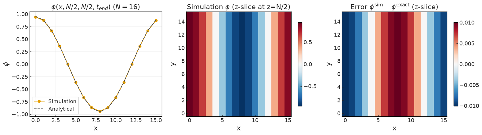
N=16: simulation phi range = [-0.9418, 0.9418], analytical decay factor = 0.9518, max pointwise error = 1.007e-02

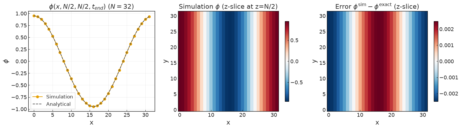
N=32: simulation phi range = [-0.9494, 0.9494], analytical decay factor = 0.9518, max pointwise error = 2.488e-03

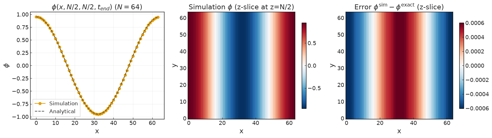
N=64: simulation phi range = [-0.9512, 0.9512], analytical decay factor = 0.9518, max pointwise error = 6.022e-04

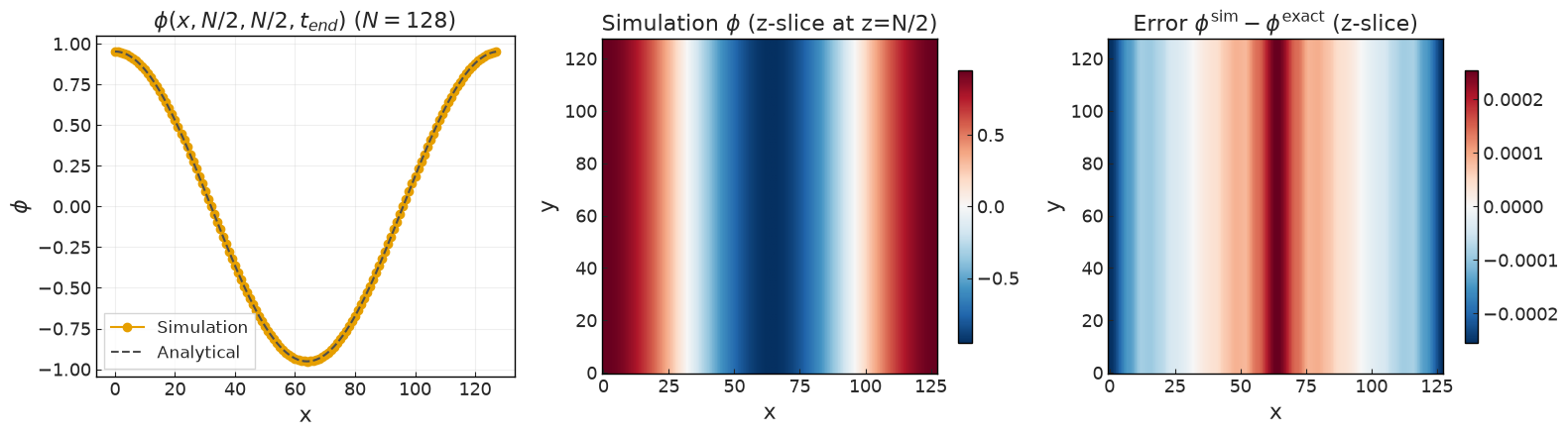
N=128: simulation phi range = [-0.9516, 0.9516], analytical decay factor = 0.9518, max pointwise error = 2.544e-04

\(\phi\) \(L_2\)-norm decay over time

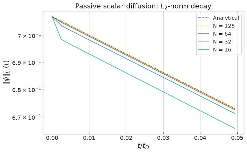
The volume-averaged \(L_2\) norm \(\|\phi(\cdot, t)\|_{L_2}\) should follow the analytical exponential decay \((\phi_0 / \sqrt{2}) \, e^{-D k^2 t}\), where the \(\sqrt{2}\) is the L2 norm of \(\cos(kx)\) over the periodic interval. Plotting on a log y-axis gives a straight line whose slope is \(-D k^2\).

fig, ax = plt.subplots(figsize=(8, 5))

for i, N in enumerate(GRID_SIZES[::-1]):
    if N not in data:
        continue
    t_arr = data[N]["times"]
    phi_l2_sim = data[N]["phi_l2"]
    k = 2.0 * np.pi / N
    t_decay = 1.0 / (D_LBM[N] * k**2)
    t_norm = t_arr / t_decay
    phi_l2_exact = np.array([phi_l2_norm_analytical(t, N, D_LBM[N], PHI_AMPLITUDE) for t in t_arr])
    if i == 0:
        ax.semilogy(
            t_norm,
            phi_l2_exact,
            **common.markers.exp_line(linestyle="--"),
            label="Analytical",
        )
    ax.semilogy(t_norm, phi_l2_sim, label=f"N = {N}", alpha=0.7)

ax.set_xlabel(r"$t / t_D$")
ax.set_ylabel(r"$\|\phi\|_{L_2}(t)$")
ax.set_title(r"Passive scalar diffusion: $L_2$-norm decay")
ax.legend()
plt.tight_layout()
plt.show()

Measured decay rate vs analytical

Fitting \(\log\|\phi\|_{L_2}(t) = a - \lambda t\) on each grid and comparing the fitted \(\lambda_{\text{lbm}}\) to the analytical \(\lambda_{\text{exact}} = D k^2\). Spatial truncation should not affect the decay rate to leading order, so the match is expected to be tight on every grid.

print(f"{'N':>4}  {'lambda_exact':>14}  {'lambda_lbm':>14}  {'rel_err':>10}")
for N in GRID_SIZES:
    if N not in data:
        continue
    t_arr = data[N]["times"]
    phi_l2_sim = data[N]["phi_l2"]
    mask = phi_l2_sim > 0
    if mask.sum() < 2:
        continue
    slope, _ = np.polyfit(t_arr[mask], np.log(phi_l2_sim[mask]), 1)
    lam_lbm = -slope
    lam_exact = D_LBM[N] * (2 * np.pi / N) ** 2
    rel = abs(lam_lbm - lam_exact) / lam_exact
    print(f"{N:>4d}  {lam_exact:>14.6e}  {lam_lbm:>14.6e}  {rel:>10.2%}")

   N    lambda_exact      lambda_lbm     rel_err
  16    3.855314e-05    4.120339e-05       6.87%
  32    1.927657e-05    1.961095e-05       1.73%
  64    9.638286e-06    9.673127e-06       0.36%
 128    4.819143e-06    4.826055e-06       0.14%

Summary

A passing result shows:

1. The \(L_2\) scalar error decreases with grid refinement, with all errors well below 1%.

2. The convergence order between consecutive levels is close to 2, confirming second-order spatial accuracy of the D3Q7 RR-BGK scalar scheme.

3. The \(L_2\) norm \(\|\phi(\cdot, t)\|_{L_2}\) tracks the exact analytical decay curve on every grid.

4. The fitted decay rate \(\lambda_{\text{lbm}}\) matches the analytical \(\lambda_{\text{exact}} = D k^2\) to within a few percent (relative error smaller than the spatial truncation error).

Flow field

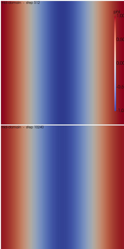
Scalar field on the mid-domain plane (plane_series.mid_z) of the finest grid (N = 128): the cosine mode at the first and last exported steps, showing the diffusive decay.

from nassu import viz

viz.enable_offscreen()

PANEL = (520, 520)
cfg = sim_cfgs["passiveScalarDiffusion3D", 3]  # N = 128
source = viz.PlaneSource.from_cfg(cfg, series="plane_series", plane="mid_z")
view = viz.frame_domain((128.0, 128.0, 128.0), "z", panel=PANEL, slice_coord=64.0)

steps = [source.steps[0], source.steps[-1]]
plotter = viz.render_grid(
    [viz.Panel("mid-domain", source, view)],
    steps=steps,
    scalar="scalar_phi",
    cmap="coolwarm",
    clim=(-1.0, 1.0),
    bar_title="phi",
    panel_size=PANEL,
)
plotter.show()

2026-06-29 14:43:46.276 (   3.602s) [    7FA065DB5740]vtkXOpenGLRenderWindow.:1460  WARN| bad X server connection. DISPLAY=
/tmp/ipykernel_1968349/1281523554.py:20: UserWarning: Using static image for notebook display.
Install trame for interactive backends: pip install "pyvista[jupyter]"
  plotter.show()

Version

sim_info = sim_cfgs_list[0].output.read_info()

nassu_commit = sim_info["commit"]
nassu_version = sim_info["version"]
print("Version:", nassu_version)
print("Commit hash:", nassu_commit)

Version: 2.0.1a0
Commit hash: 80a1135356dcbcdac92068bde45adb0fae958657

Configuration

from IPython.display import Code

Code(filename=filename)

# Passive scalar transport - 3D pure-diffusion convergence
#
# Validates the scalar advection-diffusion (DDF) module against the exact
# analytical solution for a single Fourier mode diffusing on a periodic
# domain with a stationary fluid. Four grid resolutions (N = 16, 32, 64,
# 128) are run with TGV-style scaling: tau-0.5 proportional to N (so
# D_lbm scales with N), and n_steps proportional to N. The Fourier
# number Fo = D_phys * t_phys / L_phys^2 = D_lbm * k_lbm^2 * n_steps is
# constant across grids (~4.9%), keeping the same physical diffusion
# extent at every resolution.
#
# Initial scalar field (cosine mode along x):
#   phi(x, y, z, 0) = cos(2*pi*x/N)
#   k = 2*pi/N
#
# Analytical solution (pure diffusion):
#   phi(x, y, z, t) = cos(k x) * exp(-D k^2 t)
#
# The fluid is stationary (u=0, rho=1) and stays at the equilibrium
# fixed point of the LBE. Per-grid scalar tau matches TGV's ramp
# 0.501 -> 0.508 (cs2_phi = 1/4 for D3Q7, so D = (tau-0.5)/4).
#
# Error metric: normalised L2 phi error at t_end. Expected convergence:
# O(dx^2) on a log-log plot.

simulations:
  - name: passiveScalarDiffusion3D
    save_path: ./validation/scalar_transport/01_passive_scalar_transport/results/passive_scalar_diffusion

    n_steps: !unroll [1280, 2560, 5120, 10240]

    report:
      frequency: 1000

    domain:
      domain_size:
        x: !unroll [16, 32, 64, 128]
        y: !unroll [16, 32, 64, 128]
        z: !unroll [16, 32, 64, 128]
      block_size: 8

    data:
      exports:
        default:
          macrs: [rho, u, scalar_phi, scalar_q_neq]
          interval:
            frequency: !unroll [64, 128, 256, 512]
            lvl: 0
          target:
            volume: {}
          outputs:
            instantaneous: true
        plane_series:
          macrs: [scalar_phi]
          interval: {frequency: !unroll [64, 128, 256, 512], lvl: 0}
          target:
            planes:
              # Mid-domain cross-section of the decaying cosine mode.
              mid_z:
                axis: z
                axis_pos: !unroll [8, 16, 32, 64]
                dist: 1
          outputs:
            instantaneous: true

    models:
      precision:
        default: single

      LBM:
        # Fluid stays at the equilibrium fixed point (u=0, rho=1); tau
        # only matters for damping numerical noise, so it is held at a
        # safely-stable 0.6 across all grids. The TGV-style ramp applies
        # only to the *scalar* diffusivity below.
        tau: 0.6
        vel_set: D3Q27
        coll_oper: RRBGK

      engine:
        name: CUDA

      BC:
        periodic_dims: [true, true, true]

      # Single passive scalar `scalar` (no buoyancy or other fluid
      # coupling). D in lattice units follows tau-0.5 = N / 16000 with
      # cs2_phi = 1/4: D = (tau-0.5)/4 -> 0.00025, 0.0005, 0.001, 0.002.
      scalar_transports:
        scalar:
          velocity_set: D3Q7
          collision_operator: RRBGK
          adv_diff_equation:
            D: !unroll [0.00025, 0.0005, 0.001, 0.002]
            S: "0"
          initial_field: !unroll
            - "cos(2 * pi * x / 16)"
            - "cos(2 * pi * x / 32)"
            - "cos(2 * pi * x / 64)"
            - "cos(2 * pi * x / 128)"