Wall-model boundary-layer inertia and filtering¶

This page is the capstone of the wall-model chapter. The earlier pages built a ladder of wall-stress models that assume the near-wall layer is quasi-steady, re-equilibrating instantly at every step. That assumption is what lets the TBL model solve an algebraic, memory-less system each step. The price is that, coupled to an unsteady, weakly-compressible LBM host, the model can resonate with the solver’s acoustic channel: it reads acoustic pressure noise as if it were a hydrodynamic gradient, and it injects step changes in wall stress that radiate fresh acoustic noise back. The fix is to give the modeled boundary layer the physical inertia it actually has, filtering the input and relaxing the output so the wall stress responds on a finite, node-local timescale instead of instantaneously. The remainder of this page derives that mechanism and the parameters that control it.

Key idea: give the modeled layer its physical inertia

The quasi-steady assumption makes the TBL solve cheap but also memory-less, and a memory-less wall model coupled to a weakly-compressible LBM closes a feedback loop with the acoustic channel. Restoring the boundary-layer inertia breaks the loop: filter the pressure-gradient input so acoustic noise is not read as a hydrodynamic gradient, and relax the friction-velocity output so the wall stress changes on a finite node-local timescale instead of jumping every step.

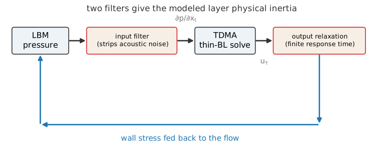
../../_images/wm_pressure_filter_loop.svg — The wall-model pressure-gradient loop. The LBM pressure passes an input filter that removes acoustic noise before the tangential gradient enters the TDMA solve; the resulting friction velocity passes an output relaxation filter that gives the modeled layer a finite response time instead of jumping each step, before the wall stress is returned to the flow.¶

The TBL-based wall models (EqTBL and NonEqTBL) solve a steady-state boundary-layer ODE at every LBM step. Because the host LBM is unsteady and weakly compressible, this raises two coupling issues that, left unaddressed, drive a feedback loop between the wall model and the LBM acoustic channel.

Input side. The non-equilibrium TBL wall model feeds the streamwise pressure-gradient term \((1/\rho)\,\partial p/\partial x_t\) of (5) into the TDMA solve. Pressure in LBM is tied algebraically to density (\(p = \rho c_s^2\)), so the gradient signal picks up acoustic density fluctuations alongside the hydrodynamic content the ODE actually requires. At the typical CWE lattice Mach \(\mathrm{Ma}_{\mathrm{lattice}} \sim 0.05 - 0.1\) the acoustic perturbations can be substantially larger than the hydrodynamic gradient. Feeding the raw signal into the TDMA contaminates the friction velocity \(u^{*}\) and amplifies the loop.

Output side. The TDMA is algebraic in time - every step it produces an instantaneous equilibrium solution for \(u^{*}\) consistent with the matching-point state, with no memory of the previous step. In a real boundary layer the wall stress cannot re-equilibrate instantaneously; there is a finite inertial timescale set by the fluid layer between the wall and the matching point. A step change in TDMA-output \(u^{*}\) between adjacent kernel steps becomes a step change in the IBM body force, which radiates as artificial acoustic content into the LBM. That acoustic content then returns to the IBM nodes as density perturbations, closing the loop.

Both issues are addressed by the same physical idea: introduce the boundary-layer inertia explicitly into the wall-model coupling. The input side is filtered per Lagrangian node before \(\partial p/\partial x_t\) reaches the TDMA; the output side relaxes \(u^{*}\) toward the TDMA’s instantaneous solution instead of taking it directly. Both filters share a single node-local timescale derived from the matching-point state, so faster-responding nodes get lighter filtering and quiescent ones get heavier filtering. The construction follows the Lagrangian relaxation framework for wall stress proposed by Fowler et al.[1]. No global filter coefficient is exposed; the only user-facing knobs are a floor on the friction velocity used by the adaptation and a static loop-gain multiplier applied to the filtered pressure-gradient signal before it enters the TDMA.

Parameters¶

Two parameters on the NonEqTBL wall model control the filter:

NeqWM_u_friction_floor: Lower bound on the friction velocity used internally to adapt the smoothing strength. Default 1e-4 (lattice units). A case-specific guideline is one tenth of the log-law equilibrium friction velocity at the freestream scale, \(\kappa\,U_\infty/[10\,\ln(h_{\mathrm{wm}}/z_0)]\). The floor does not clamp the TDMA output; it only keeps the adaptive coefficient well-defined.
NeqWM_pres_grad_mult: Static multiplier \(m \in [0, 1]\) applied to the filtered pressure gradient before it enters the TDMA. Default 1.0 leaves the wall model unchanged. Setting it to 0.0 zeroes the pressure-gradient source seen by the TDMA (NonEqTBL then reduces to the equilibrium TBL) while pres_grad and pres_grad_filt keep updating on every Lagrangian node, which is useful for spectral diagnostics in passive-sensor mode. The recommended setting is a Mach-derived value; see Physical interpretation: Mach-derived multiplier.

Physical interpretation: Mach-derived multiplier¶

Why this is not just a tuning knob

For weakly-compressible LBM, NeqWM_pres_grad_mult has a definite physical meaning that fixes its natural value at \(m = \mathrm{Ma}_{\mathrm{LBM}}\). The reason: LBM ties pressure to density, so the raw \(\partial p/\partial x_t\) signal carries acoustic content that overspecifies the incompressible source term the TBL ODE expects by a factor of \(1/\mathrm{Ma}_{\mathrm{LBM}}\). Multiplying by \(\mathrm{Ma}_{\mathrm{LBM}}\) rescales the magnitude back to what an incompressible solver would deliver. Needing a value below \(\mathrm{Ma}_{\mathrm{LBM}}\) signals the loop is hotter than the Mach mismatch alone explains.

The multiplier NeqWM_pres_grad_mult looks like a tuning knob, but for weakly-compressible LBM it has a definite physical meaning that fixes a “natural” value.

LBM ties pressure to density (\(p = \rho c_s^2\)), so the \(\partial p / \partial x_t\) signal the wall model reads contains both a hydrodynamic and an acoustic contribution. In lattice units their magnitudes scale as

(1)¶\[ \delta p_{\mathrm{hydro}} \sim \rho\, U^2 \;=\; \mathrm{Ma}_{\mathrm{LBM}}^2 \,\rho\, c_s^2, \qquad \delta p_{\mathrm{acou}} \sim \rho\, c_s\, u_{\mathrm{acou}} \;\sim\; \mathrm{Ma}_{\mathrm{LBM}} \,\rho\, c_s^2, \]

with \(\mathrm{Ma}_{\mathrm{LBM}} = U_{\mathrm{LBM}}/c_s\) and \(c_s = 1/\sqrt{3}\). The ratio is

(2)¶\[ \frac{\delta p_{\mathrm{acou}}}{\delta p_{\mathrm{hydro}}} \;\sim\; \frac{1}{\mathrm{Ma}_{\mathrm{LBM}}}, \]

so the acoustic component dominates the raw signal in lattice units by a factor of \(1/\mathrm{Ma}_{\mathrm{LBM}}\).

In a true incompressible TBL formulation - which is what the TBL ODE in (5) is - \(\partial p/\partial x_t\) means the hydrodynamic component alone. Feeding the LBM total signal without correction overspecifies the source term by \(1/\mathrm{Ma}_{\mathrm{LBM}}\).

The static multiplier \(m\) corrects the magnitude of the signal back to the incompressible expectation. Setting

(3)¶\[ m \;=\; \mathrm{Ma}_{\mathrm{LBM}} \;=\; \frac{U_{\mathrm{LBM}}}{c_s} \;=\; U_{\mathrm{LBM}}\,\sqrt{3} \]

gives

\[ m \cdot \big(\delta p_{\mathrm{hydro}} + \delta p_{\mathrm{acou}}\big) \;\sim\; \mathrm{Ma}_{\mathrm{LBM}} \cdot \delta p_{\mathrm{acou}} \;\sim\; \delta p_{\mathrm{hydro}}, \]

i.e. the average pressure-gradient magnitude reaching the TDMA matches the hydrodynamic component that an incompressible solver would deliver at the same flow conditions.

This is a magnitude-only correction: a single scalar \(m\) cannot separate the hydrodynamic from the acoustic content (that is the job of the input filter on the spectral axis). It does rescale the overall amplitude so the TBL ODE operates on a signal of the right order of magnitude. The two corrections compose: the input filter removes the high-frequency acoustic energy in the spectrum, and \(m = \mathrm{Ma}_{\mathrm{LBM}}\) rescales what remains so the hydrodynamic component reaches the TDMA at its physically correct amplitude.

A typical CWE setup with \(U_{\mathrm{LBM}} = 0.05\) gives \(m \approx 0.087\); with \(U_{\mathrm{LBM}} = 0.1\), \(m \approx 0.17\). The case YAML can derive this automatically:

variables:
  u_inf_lattice: 0.05
  Ma_LBM: !math ${u_inf_lattice} * (3 ** 0.5)

simulations:
  - name: ...
    models:
      IBM:
        body_cfgs:
          sphere_cfg:
            wall_model:
              params:
                NeqWM_pres_grad_mult: !math ${Ma_LBM}

If loop stability requires going below \(\mathrm{Ma}_{\mathrm{LBM}}\), that indicates the closed wall- model loop is hotter than the Mach mismatch alone explains and the extra attenuation is acting as a loop-gain knob, not a magnitude correction.

Start-up and integration¶

The input filter state is zero-initialised on each Lagrangian node, so the source seen by the TDMA ramps up from zero at the rate set by the boundary-layer state at that node. The output relaxation similarly uses the previous step’s u_friction (zero on the very first wall-model step) and the floor as the starting point. Both are independent of the IBM FORCES_ACCOMODATE_TIME ramp; all three mechanisms compose when active. No additional state field is added to the IBM node struct - the only persisted quantities are u_friction (already written by the TDMA and exported to the IBM XDMF stream) and pres_grad_filt.

The output relaxation is applied uniformly to every wall model (EqLog, EqTBL, NonEqTBL), since the same physical argument holds: any per-step algebraic solve - whether the log-law formula or the TBL TDMA - introduces a step change in \(u^{*}\) between adjacent kernel calls. The coefficient is derived once per Lagrangian node from the lagged friction velocity and shared with the input filter, so faster-responding nodes get lighter filtering on both sides.