Physical and Lattice Units

Every equation in this chapter is written in lattice units: the grid spacing and the time step are both set to one, \(\Delta x = \Delta t = 1\). This is the most user-facing convention in the solver, and the most common source of confusion. This page explains why it is done, how to convert between the physical world and the lattice, and how to choose the three free numbers (\(\tau\), \(\Delta x\), \(\Delta t\)) so that a simulation is both correct and stable. It closes with a fully worked computational wind engineering example.

The unit relations here follow the standard treatment in Krüger et al.[1].

Why lattice units?

The lattice Boltzmann algorithm streams populations exactly one node per time step. That is only clean if the node spacing and the time step are the natural units of the scheme. Setting \(\Delta x = \Delta t = 1\) removes them from every formula, so the speed of sound becomes the fixed constant \(c_s = 1/\sqrt{3}\) and the relaxation frequency \(\omega\) is a pure number. The solver therefore works entirely in these dimensionless units, and your job at setup time is to build the bridge between them and metres and seconds.

The bridge rests on a principle from dimensional analysis: two flows are dynamically identical if their dimensionless groups match. For the incompressible flows Nassu targets, the governing group is the Reynolds number. Match the Reynolds number between the physical problem and the lattice, keep the Mach number small enough that compressibility error is negligible, and the lattice solves your physical problem.

Note

A dimensionless group is a ratio of physical quantities whose units cancel, so it takes the same value in any unit system. The Reynolds number \(\mathrm{Re} = UL/\nu\) compares inertial to viscous forces and is the group that sets whether a flow is laminar or turbulent; the Mach number \(\mathrm{Ma} = U/c_s\) compares the flow speed to the speed of sound. Matching them between the physical flow and the lattice is what dynamic similarity guarantees.

Conversion factors

Convert with one factor per independent dimension. Choose a reference length, a reference velocity and a reference density; the rest follow. Denote physical quantities with a subscript \(p\) and lattice quantities with no subscript.

(1)\[ C_x = \frac{L_p}{L}, \qquad C_u = \frac{U_p}{U}, \qquad C_\rho = \frac{\rho_p}{\rho} \]

Here \(C_x\) is the length of one lattice spacing in metres, \(C_u\) is the speed represented by one lattice velocity unit, and \(C_\rho\) fixes the mass scale (commonly \(\rho = 1\) in lattice units, so \(C_\rho = \rho_p\)). Every other conversion factor is a product of these three:

(2)\[ C_t = \frac{C_x}{C_u}, \qquad C_\nu = \frac{C_x^2}{C_t} = C_x\, C_u, \qquad C_p = C_\rho\, C_u^2 \]

with \(C_t\) the duration of one time step, \(C_\nu\) the viscosity factor and \(C_p\) the pressure factor. A physical quantity equals its lattice value times the corresponding factor, for example \(\nu_p = C_\nu\, \nu\).

Note

Density usually drops out of incompressible results, since forces and pressures of engineering interest are reported as dimensionless coefficients. The two factors that matter most in practice are \(C_x\) and \(C_u\).

The two dimensionless constraints

Two numbers decide whether a chosen set of lattice parameters is usable.

Reynolds number (accuracy). The Reynolds number must be identical in both systems, because it is the group that governs the flow:

(3)\[ \mathrm{Re} = \frac{U_p L_p}{\nu_p} = \frac{U L}{\nu} \]

This is the equation you actually solve at setup time. Pick the lattice resolution \(L\) (in nodes) and a lattice velocity \(U\), and (3) fixes the lattice viscosity \(\nu = U L / \mathrm{Re}\). The viscosity-relaxation relation from the Chapman-Enskog derivation, (10), then fixes the relaxation time:

(4)\[ \nu = c_s^2 \left(\tau - \frac{1}{2}\right) \quad\Longrightarrow\quad \tau = \frac{1}{2} + \frac{\nu}{c_s^2} = \frac{1}{2} + 3\nu \]

using \(c_s^2 = 1/3\) and \(\Delta t = 1\).

Mach number (stability and compressibility). The lattice velocity is not free to be large. The weakly-compressible analysis of the Chapman-Enskog page bounds the Mach number:

(5)\[ \mathrm{Ma} = \frac{U}{c_s} = \sqrt{3}\, U < 0.1 \]

A common, safe choice is to keep the lattice velocity around \(U \approx 0.05\) or below, which gives \(\mathrm{Ma} \approx 0.09\) and keeps the density fluctuations (\(\sim \mathrm{Ma}^2\)) at the percent level.

Warning

The lattice Mach number is a binding accuracy and compressibility constraint, not a soft guideline. Raising \(U\) to shrink the node count drives \(\mathrm{Ma}\) up quickly, and beyond \(\mathrm{Ma} \approx 0.1\) the spurious density fluctuations (\(\sim \mathrm{Ma}^2\)) and the \(\mathcal{O}(\mathrm{Ma}^3)\) equilibrium truncation error stop being negligible. Keep \(\mathrm{Ma} < 0.1\).

These two constraints pull against each other and define the central trade-off of setting up an LBM run:

• A smaller lattice velocity \(U\) reduces compressibility error, but lowers the lattice viscosity for a fixed Reynolds number, pushing \(\tau\) toward the stability limit \(\tau = 0.5\) (\(\omega \to 2\)).

• A finer grid (larger \(L\) in nodes) raises the lattice viscosity for a fixed Reynolds number, moving \(\tau\) to a safer value, at the cost of more nodes and time steps.

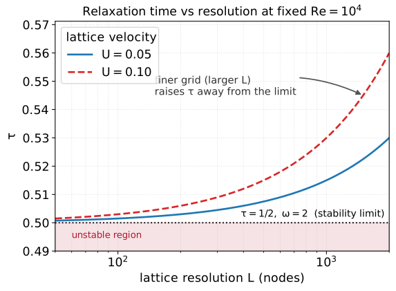
For a fixed Reynolds number, refining the grid (larger \(L\)) and raising the lattice velocity \(U\) both lift the relaxation time \(\tau\) away from the stability limit \(\tau = 1/2\); the curves use \(\mathrm{Re} = 10^4\) for legibility.

The collision operator chosen matters here: as discussed on the collision operators page, the regularized RR-BGK operator used by Nassu remains stable very close to \(\omega = 2\), which is what makes high-Reynolds simulations affordable.

A frequent question: the CFL number

Engineers arriving from finite-volume or finite-difference solvers almost always ask which Courant number an LBM run uses, since there the CFL condition is the binding stability limit that ties the time step to the grid spacing. In the lattice Boltzmann method the answer is immediate. Because \(\Delta x = \Delta t = 1\) at every refinement level, the Courant number collapses to the lattice velocity itself:

(6)\[ \mathrm{CFL} = \frac{|u|\,\Delta t}{\Delta x} = |u| \]

The reason there is no separate CFL stability limit is that streaming is an exact shift of exactly one node per time step, not a numerical approximation of advection: a population leaving a node lands precisely on its neighbour, with no interpolation and no truncation. The time step is therefore not a free knob to be tuned against a Courant ceiling, as it is in an explicit Navier-Stokes discretization. Instead the lattice velocity is bounded by the Mach constraint (5), \(|u| < 0.1/\sqrt{3} \approx 0.058\), so an LBM simulation automatically runs at a very low effective Courant number.

Note

The flip side is that resolution in space and in time cannot be chosen independently. Halving \(\Delta x\) (a finer grid) halves \(\Delta t\) as well, because the two are locked together by \(\Delta x = \Delta t = 1\) in lattice units. This is exactly the 2:1 space-time ratio used at every multiblock refinement level: a block with half the grid spacing also takes two time steps for every one of its coarser neighbour.

Choosing the parameters: the recipe

For a given physical problem the practical workflow is:

1. Compute the physical Reynolds number \(\mathrm{Re} = U_p L_p / \nu_p\).

2. Choose the lattice resolution \(L\) (nodes across the reference length). This is your accuracy and cost lever.

3. Choose the lattice velocity \(U\) to satisfy (5), typically \(U \lesssim 0.05\).

4. Compute the lattice viscosity from the matched Reynolds number, \(\nu = U L / \mathrm{Re}\).

5. Compute the relaxation time from (4) and check that \(\tau\) is comfortably above \(0.5\).

6. Recover the conversion factors (1) and (2) to translate results back to physical units.

Worked example: flow around a tall building

Consider a representative computational wind engineering case: wind around a tall building.

Physical data.

• Reference length (building width): \(L_p = 50\,\text{m}\) - the scale that sets the dominant vortex shedding.

• Reference velocity (mean wind at building height): \(U_p = 30\,\text{m/s}\) - a strong-wind design condition.

• Air kinematic viscosity: \(\nu_p = 1.5\times 10^{-5}\,\text{m}^2/\text{s}\).

The physical Reynolds number is

(7)\[ \mathrm{Re} = \frac{U_p L_p}{\nu_p} = \frac{30 \times 50}{1.5\times 10^{-5}} = 1.0\times 10^{8} \]

This is a very high Reynolds number, which is exactly why an LES with a turbulence model (and, near walls, a wall model) is used rather than a direct simulation; this is the regime and the modelling strategy for which Nassu is designed [2].

Lattice choices.

• Resolve the building width with \(L = 100\) nodes - a coarse but illustrative choice; production runs use more, often with multiblock refinement to concentrate nodes near the body.

• Set the lattice velocity to \(U = 0.05\) - giving \(\mathrm{Ma} = \sqrt{3}\times 0.05 \approx 0.087 < 0.1\), safely weakly compressible.

Derived lattice viscosity and relaxation time. Matching the Reynolds number,

(8)\[ \nu = \frac{U L}{\mathrm{Re}} = \frac{0.05 \times 100}{1.0\times 10^{8}} = 5.0\times 10^{-8} \]

(9)\[ \tau = \frac{1}{2} + 3\nu = 0.5 + 3\times 5.0\times 10^{-8} \approx 0.50000015 \]

The relaxation time sits extremely close to the stability limit \(0.5\). This is the honest signal that a plain BGK collision would be unusable here and that in this under-resolved high-Reynolds regime a stabilized, regularized operator together with an LES subgrid viscosity is required. It also shows why refining the grid (raising \(L\)) is the standard lever: doubling \(L\) doubles \(\nu\) and moves \(\tau\) away from the limit.

Converting results back. The conversion factors are

(10)\[ C_x = \frac{L_p}{L} = \frac{50}{100} = 0.5\,\text{m/node}, \qquad C_u = \frac{U_p}{U} = \frac{30}{0.05} = 600\,\text{m/s per lattice unit} \]

so one time step represents

(11)\[ C_t = \frac{C_x}{C_u} = \frac{0.5}{600} \approx 8.3\times 10^{-4}\,\text{s} \]

A lattice velocity of, say, \(0.04\) read from a probe therefore corresponds to \(0.04 \times 600 = 24\,\text{m/s}\), and a shedding period measured as \(N\) time steps corresponds to \(N \times 8.3\times 10^{-4}\,\text{s}\).

The conversion in one sentence

The whole conversion hangs on two choices: the lattice resolution \(L\) and the lattice velocity \(U\). Fix those subject to \(\mathrm{Ma} < 0.1\), match the Reynolds number to get \(\nu\) and hence \(\tau\), and every other quantity follows from the factors in (1) and (2).

Next steps

This page closes the core LBM learning path: you now have the method (kinetic theory, the lattice equation, collision and regularization), the proof that it solves Navier-Stokes (Chapman-Enskog), and the unit system to drive it. From here the chapter offers one optional extension, Compressible LBM, which relaxes the strict low-Mach assumption used above to reach non-isothermal and high-Mach flows; it sits outside the weakly-compressible path this chapter is built around. For applying the method, the natural continuation is the LES chapter, which adds the subgrid model that makes high-Reynolds simulations affordable.

---

[1]

Timm Krüger, Halim Kusumaatmaja, Alexandr Kuzmin, Orest Shardt, Goncalo Silva, and Erlend Magnus Viggen. The lattice Boltzmann method. Graduate Texts in Physics. Springer International Publishing, Basel, Switzerland, 1 edition, November 2016.

[2]

Waine Oliveira, Rodrigo S. Romanus, and Alan Lugarini. Nassu: a high performance LES solver for computational wind engineering. Journal of Wind Engineering and Industrial Aerodynamics, 274:106465, 2026. doi:10.1016/j.jweia.2026.106465.