Flow Over Stationary Sphere

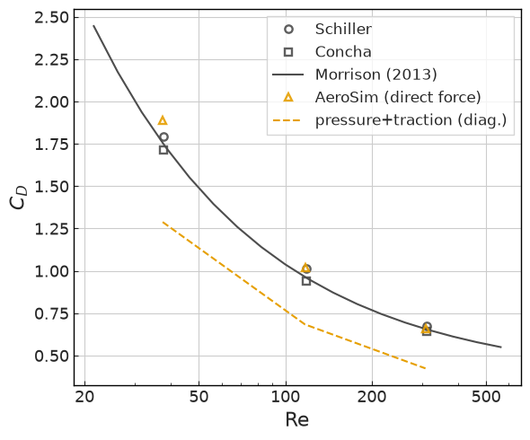
The simulation of a laminar flow over a stationary sphere is used for the validation of force spreading aspects of the immersed boundary method (IBM). For that purpose, the drag coefficient is measured through the forces calculated at the Lagrangian mesh.

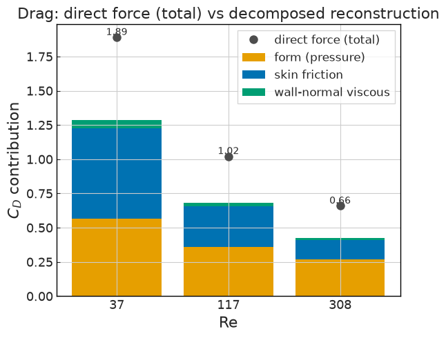
Total drag from the direct IBM force. The sphere drag reported below is the full drag (form pressure + skin friction), obtained by summing the IBM spreading force the solver applied to enforce the no-slip condition over the body’s Lagrangian nodes (nassu.viz.read_body_ibm_force). Each node’s force is rescaled from its level-local lattice units to global units - a (2^-lvl)^2 factor, the dx^2 area ratio - before summing (issue #1016). This direct force needs no surface-pressure or wall-stress reconstruction and matches the reference correlations to within a few percent. The decomposed pressure + viscous-traction route (nassu.viz.pressure_force_coefficients + nassu.viz.force_coefficients) is kept only as a diagnostic split; on this sphere it under-predicts the total by ~30%.

from nassu.cfg.model import ConfigScheme

filename = "validation/external_aero/01_flow_over_sphere/01_flow_over_sphere.nassu.yaml"

sim_cfgs = ConfigScheme.sim_cfgs_from_file_dct(filename)

A multilevel configuration is adopted to allow a large ratio between the sphere’s and domain’s sizes.

sim_laminar = [sim_cfg for (name, _), sim_cfg in sim_cfgs.items() if name.startswith("laminar")]
sim_turb = next(
    sim_cfg for (name, _), sim_cfg in sim_cfgs.items() if name == "turbulentFlowOverSphere"
)
sim_turb_les = next(sim_cfg for (name, _), sim_cfg in sim_cfgs.items() if name.endswith("LES"))
sim_cfgs_use = sim_laminar + [sim_turb] + [sim_turb_les]

Functions to use for flow over sphere processing

import pathlib

import numpy as np
import pandas as pd

import nassu.viz as viz
from nassu.cfg.schemes.simul import SimulationConfigs


def get_experimental_profile_Cp(reynolds: float) -> pd.DataFrame:
    files_tau: dict[float, str] = {
        4200: "Cp_vs_theta_Re_4200.csv",
        50000: "Cp_vs_theta_Re_50000.csv",
        300000: "Cp_vs_theta_Re_300000.csv",
        400000: "Cp_vs_theta_Re_400000.csv",
        1140000: "Cp_vs_theta_Re_1140000.csv",
    }
    filename = (
        pathlib.Path("validation/external_aero/01_flow_over_sphere/reference")
        / files_tau[reynolds]
    )
    # ([theta], [Cp])
    return pd.read_csv(filename, delimiter=",")


def get_experimental_profile_Cd() -> pd.DataFrame:
    filename = (
        pathlib.Path("validation/external_aero/01_flow_over_sphere/reference")
        / "drag_coefficient.csv"
    )
    # ([Author], [Re], [Cd])
    return pd.read_csv(filename, delimiter=",")


def mean_pressure_form_drag(
    sim_cfg: SimulationConfigs,
    *,
    u_inf: float,
    normal: np.ndarray,
    area: np.ndarray,
    a_ref: float,
    rho_inf: float = 1.0,
    body_name: str = "sphere",
    series: str = "default_series",
    stats_start: float = 0.0,
):
    """Time-mean form (pressure) drag/lift coefficients from a body pressure series.

    Reads the surface-density history sampled over the body nodes, forms the
    per-node mean ``Cp = (rho - rho_inf) / (1.5 rho_inf u_inf**2)`` and integrates
    the pressure force ``C_F = -sum_i Cp_i n_i A_i / a_ref`` over the sphere with
    ``nassu.viz.pressure_force_coefficients``. The per-node outward ``normal`` and
    ``area`` come from the ``body_nodes`` friction export, which shares the exact
    same deterministic per-triangle ordering as the surface-pressure series (both
    keyed by the body-node index), so the form and viscous drag use identical
    geometry weights and add to the full drag. Returns ``(Cd_pressure, Cl_pressure)``.
    """
    hs = sim_cfg.output.exports[series].series.bodies[body_name]
    df = hs.read_full_data("rho")
    df = df[df["time_step"] >= stats_start].drop(columns="time_step")
    rho_mean = df.mean().to_numpy()  # (n_nodes,), body-node index order

    assert len(rho_mean) == len(area) == len(normal), (len(rho_mean), len(area), len(normal))
    cp = (rho_mean - rho_inf) / (1.5 * rho_inf * u_inf**2)
    coeffs = viz.pressure_force_coefficients(cp, normal, area, a_ref=a_ref)
    return float(coeffs["Cd_pressure"]), float(coeffs["Cl_pressure"])

Results

The drag coefficient reported here is the total drag from the direct IBM force: the spreading force summed over the sphere’s Lagrangian nodes (form pressure + skin friction together), matching the Schiller / Concha / Morrison correlations to within a few percent across the Reynolds sweep. The decomposed pressure + viscous-traction reconstruction is overlaid as a diagnostic; it systematically under-predicts the total by ~30% (issue #1016). The stacked bar shows the reconstruction split (form + friction + wall-normal viscous) with the direct-force total marked, so the shortfall is visible per Reynolds number.

import matplotlib.pyplot as plt

import nassu.viz as common

common.use_style()

fig, ax = common.fig_single()

df_exp = get_experimental_profile_Cd()
authors = ["Schiller", "Concha"]
exp_shapes = ["o", "s"]
for author, shape in zip(authors, exp_shapes):
    ax.plot(df_exp["Re"], df_exp[author], **common.markers.exp(shape=shape), label=author)

# Continuous standard-drag reference (Morrison 2013 correlation), restricted to
# the laminar sweep's Reynolds range for a like-for-like overlay.
df_morrison = pd.read_csv(
    "validation/external_aero/01_flow_over_sphere/reference/sphere_drag_Cd_vs_Re.csv",
    comment="#",
)
m = (df_morrison["Re"] >= 20) & (df_morrison["Re"] <= 600)
ax.plot(
    df_morrison["Re"][m],
    df_morrison["Cd"][m],
    **common.markers.exp_line(linestyle="-"),
    label="Morrison (2013)",
)

# TOTAL drag from the DIRECT IBM force (issue #1016): the spreading force the
# solver applied to the fluid to enforce no-slip, summed over the sphere's
# Lagrangian nodes (form pressure + skin friction together, no reconstruction).
# `nassu.viz.read_body_ibm_force` rescales each node's force from its level-local
# lattice units to global units - (2^-lvl)^2, the dx^2 area ratio - and sums it;
# `body_force_coefficients` normalizes by q*A_ref. On this sphere the direct force
# matches Schiller / Concha / Morrison to within a few percent, whereas the
# decomposed pressure + viscous-traction reconstruction (overlaid as a diagnostic
# curve, and split in the bar chart below) under-predicts the total by ~30%.
RHO_INF = 1.0
num_vals = {
    "Re": [],
    "Cd_direct": [],
    "Cd_pressure": [],
    "Cd_viscous": [],
    "Cd_friction": [],
    "Cd_normal_viscous": [],
}
for sim_cfg in sim_laminar:
    bf = common.read_body_friction(sim_cfg, "sphere", series="friction")

    # Shared reference geometry (frontal area) from the source-triangle centroids.
    diameter = float(np.ptp(bf.centroid[:, 0]))
    a_ref = np.pi * diameter**2 / 4

    # Freestream speed from the inlet BC (lattice units).
    u_inf = max(bc.ux for bc in sim_cfg.models.BC.BC_map if "ux" in bc.model_dump())
    reynolds = u_inf * diameter / sim_cfg.models.LBM.kinematic_viscosity

    # Headline total drag: the direct IBM force over the steady window.
    bif = common.read_body_ibm_force(sim_cfg, "sphere", start_step=sim_cfg.n_steps // 2)
    f_body = common.time_mean_ibm_force(bif)
    cd_direct = float(
        common.body_force_coefficients(f_body, rho_ref=RHO_INF, u_ref=u_inf, a_ref=a_ref)["Cd"]
    )

    # Diagnostic reconstruction: viscous (skin-friction + wall-normal) drag from
    # the `body_nodes` traction split, plus the form (pressure) drag from the mean
    # surface Cp. Both use the friction export's per-triangle normals/areas.
    t_mean = common.time_mean_friction(bf)
    vcoef = common.force_coefficients(
        t_mean,
        bf.normal,
        bf.area,
        rho_ref=RHO_INF,
        u_ref=u_inf,
        a_ref=a_ref,
        flow_dir=np.array([1.0, 0.0, 0.0]),
    )
    cd_viscous = float(vcoef["Cd_total"])
    cd_pressure, _ = mean_pressure_form_drag(
        sim_cfg,
        u_inf=u_inf,
        normal=bf.normal,
        area=bf.area,
        a_ref=a_ref,
        rho_inf=RHO_INF,
        series="default_series",
        stats_start=sim_cfg.n_steps // 2,
    )

    num_vals["Re"].append(reynolds)
    num_vals["Cd_direct"].append(cd_direct)
    num_vals["Cd_pressure"].append(cd_pressure)
    num_vals["Cd_viscous"].append(cd_viscous)
    num_vals["Cd_friction"].append(float(vcoef["Cd_friction"]))
    num_vals["Cd_normal_viscous"].append(float(vcoef["Cd_normal_viscous"]))

order = np.argsort(num_vals["Re"])
Re_sorted = np.array(num_vals["Re"])[order]
ax.plot(
    Re_sorted,
    np.array(num_vals["Cd_direct"])[order],
    **common.markers.sim(shape="^"),
    label="AeroSim (direct force)",
)
# Diagnostic overlay: the decomposed pressure + viscous-traction reconstruction,
# which systematically under-predicts the direct-force total (issue #1016).
recon = np.array(num_vals["Cd_pressure"])[order] + np.array(num_vals["Cd_viscous"])[order]
ax.plot(
    Re_sorted,
    recon,
    **common.markers.sim_line(linestyle="--"),
    label="pressure+traction (diag.)",
)

ax.legend()
ax.set_xscale("log")
# Log axis: plain-number ticks (the AeroSim style only covers linear axes).
common.plain_number_axis(ax, "x", ticks=[20, 50, 100, 200, 500])
ax.set_xlabel("Re")
ax.set_ylabel("$C_D$")

plt.tight_layout()
plt.show(fig)

# Drag decomposition as a STACKED BAR per Reynolds number: the reconstruction
# split into form (pressure) + skin friction + wall-normal viscous traction, with
# the DIRECT-force total (the headline Cd) drawn as a marker. The gap between the
# stack top and the marker is the reconstruction shortfall (issue #1016).
fig_dec, ax_dec = common.fig_single()
re_labels = [f"{r:.0f}" for r in Re_sorted]
pres = np.array(num_vals["Cd_pressure"])[order]
fric = np.array(num_vals["Cd_friction"])[order]
nvis = np.array(num_vals["Cd_normal_viscous"])[order]
direct = np.array(num_vals["Cd_direct"])[order]
xb = np.arange(len(re_labels))
ax_dec.bar(xb, pres, label="form (pressure)", color=common.colors.sim)
ax_dec.bar(xb, fric, bottom=pres, label="skin friction", color=common.colors.blue)
ax_dec.bar(xb, nvis, bottom=pres + fric, label="wall-normal viscous", color=common.colors.green)
ax_dec.plot(
    xb, direct, "o", color=common.colors.exp, markersize=8, label="direct force (total)", zorder=5
)
for k, tot in enumerate(direct):
    ax_dec.text(xb[k], tot, f"{tot:.2f}", ha="center", va="bottom", fontsize=10)
ax_dec.set_xticks(xb)
ax_dec.set_xticklabels(re_labels)
common.bar_axis(ax_dec)
ax_dec.set_xlabel("Re")
ax_dec.set_ylabel("$C_D$ contribution")
ax_dec.set_title("Drag: direct force (total) vs decomposed reconstruction")
ax_dec.legend()

plt.tight_layout()
plt.show(fig_dec)

/tmp/ipykernel_3072641/476860046.py:59: UserWarning: IBM node export for body 'sphere' has no `lvl` field (pre-#1016 export); rescaling all force-bearing nodes at level 1. Exact only if the body sits entirely at that level; re-run to regenerate `lvl`.
  bif = common.read_body_ibm_force(sim_cfg, "sphere", start_step=sim_cfg.n_steps // 2)
/tmp/ipykernel_3072641/476860046.py:59: UserWarning: IBM node export for body 'sphere' has no `lvl` field (pre-#1016 export); rescaling all force-bearing nodes at level 1. Exact only if the body sits entirely at that level; re-run to regenerate `lvl`.
  bif = common.read_body_ibm_force(sim_cfg, "sphere", start_step=sim_cfg.n_steps // 2)
/tmp/ipykernel_3072641/476860046.py:59: UserWarning: IBM node export for body 'sphere' has no `lvl` field (pre-#1016 export); rescaling all force-bearing nodes at level 1. Exact only if the body sits entirely at that level; re-run to regenerate `lvl`.
  bif = common.read_body_ibm_force(sim_cfg, "sphere", start_step=sim_cfg.n_steps // 2)

The pressure coefficient for the case of turbulent flow around a stationary sphere is performed for a Re=4,200 simulation to check capacity of measuring the pressure coefficient using the historic series function for a body. A posterior LES simulation is then performed for a Re=50,000 to also verify the solver stability for high Reynolds simulations. In both cases, excellent agreement with experimental data was obtained.

fig, ax = common.fig_double()


def post_proc_crossflow_sphere_Cp(
    sim_cfg: SimulationConfigs, ax, reynolds: float, u_inf: float = 0.05
):
    hs = sim_cfg.output.exports["default_series"].series.bodies["sphere"]

    df_points = pd.read_csv(hs.points_filename)
    df_hs = hs.read_full_data("rho")

    sphere_center = tuple(df_points[d].mean() for d in ("x", "y", "z"))

    # Use only points in z=0 to calculate Cp
    bool_arr = np.zeros((len(df_points),), dtype=np.bool_)
    df_points = df_points.loc[
        (df_points["z"] <= sphere_center[2] + 0.5) & (df_points["z"] >= sphere_center[2] - 0.5)
    ]
    bool_arr[df_points["idx"]] = True

    # TODO: This comes from sim_cfg, now hand written,
    # but update to calculate it automatically
    rho_inf = 1
    df_hs = df_hs[df_hs["time_step"] >= 10000]
    df_rho = df_hs.drop(columns="time_step")
    df_cp = (df_rho - rho_inf) / (1.5 * rho_inf * (u_inf**2))
    Cp_avg = df_cp.mean().to_numpy().T
    Cp_avg = Cp_avg[bool_arr]

    # Get angles for points, use acos because it goes from 0 to 180
    x = df_points["x"] - df_points.mean()["x"]
    y = df_points["y"] - df_points.mean()["y"]
    points_angles: np.ndarray = np.arccos(-x / (x**2 + y**2) ** 0.5)
    # Convert to angles
    points_angles *= 180 / np.pi
    points_angles = np.array(points_angles)

    # # Sort arrays
    argsort = points_angles.argsort()
    points_angles = points_angles[argsort]
    cp_points = Cp_avg[argsort]

    ax.plot(points_angles, cp_points, **common.markers.sim_line(linestyle="--"), label="AeroSim")

    df_exp = get_experimental_profile_Cp(reynolds)
    ax.plot(df_exp["theta"], df_exp["Cp"], **common.markers.exp(shape="o"), label="Experimental")

    ax.legend()


for i, (sim_cfg, reynolds) in enumerate([(sim_turb, 4200), (sim_turb_les, 50000)]):
    post_proc_crossflow_sphere_Cp(sim_cfg, ax[i], reynolds, u_inf=0.05)
    ax[i].set_xlim((0, 180))
    ax[i].set_ylim((-0.6, 1.2))
    ax[i].set_ylabel("$C_p$")
    ax[i].set_xlabel(r"$\theta$ (deg)")
    ax[i].set_title(f"$Re={reynolds}$")

plt.tight_layout()
plt.show(fig)

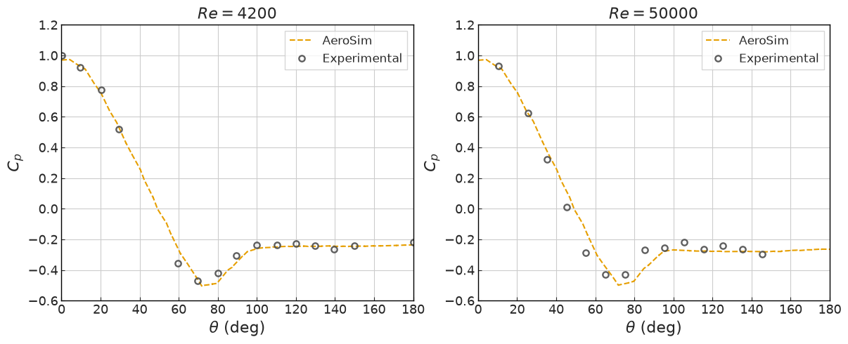
The pressure coefficient curve is very similar for both Re = 4200 and Re= 50,000. It can be seen better proximity of results in the LES simulation with a higher Reynolds number.

Force coefficients, peaks and shedding

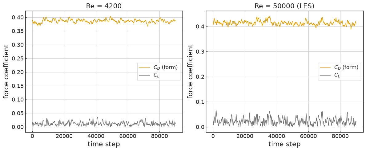
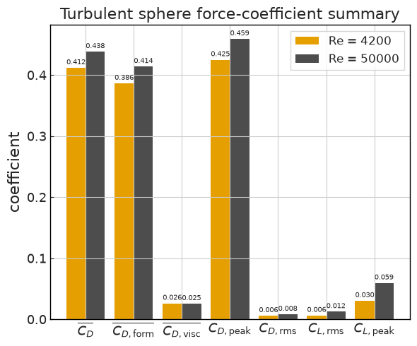
The turbulent sphere’s mean drag is the total drag from the direct IBM force (nassu.viz.read_body_ibm_force), summed over the body and rescaled per refinement level (issue #1016). The fluctuating loads and the vortex-shedding signal still come from the surface-pressure force history \(C_d(t)\), \(C_l(t)\) - the instantaneous IBM force is too noisy to resolve them - so the design peak (Cook-Mayne / Gumbel via nassu.viz.design_peak) is the pressure signal’s fluctuation lifted onto the direct mean drag, and the Strouhal number comes from the lift spectrum.

# --- Pressure-integrated force coefficients -------------------------------
# Drag and lift of the turbulent sphere are obtained by integrating the surface
# pressure over the body; the IBM spreading force is too noisy to resolve the
# fluctuating loads. For each body node i, Cp_i = (rho_i - rho_inf)/(1.5 rho_inf U^2),
# and the force-coefficient vector is C_F = -sum_i Cp_i n_i A_i / A_ref with
# A_ref = pi D^2 / 4 the frontal area. The surface pressure history comes from
# the body historic series (`default_series`); the outward unit normals and the
# per-node areas come from the `body_nodes` friction export (`bf`), which shares
# the same deterministic per-triangle ordering as the pressure series (both keyed
# by the body-node index), so the form and viscous drag use identical geometry
# weights.

U_INF = 0.05
RHO_INF = 1.0
STATS_START = 10000  # drop the initial transient (matches the Cp analysis above)


def force_coeff_series(sim_cfg, bf, body_name="sphere", series="default_series"):
    """Time series of the pressure-integrated force coefficient.

    Returns ``(time, C_F[:, 3], D)`` with ``C_F`` the (drag, y, z) coefficient
    components per exported time step and ``D`` the sphere diameter. The per-node
    outward ``normal`` and ``area`` come from the friction export ``bf``.
    """
    hs = sim_cfg.output.exports[series].series.bodies[body_name]
    df = hs.read_full_data("rho")
    df = df[df["time_step"] >= STATS_START]
    time = df["time_step"].to_numpy()
    rho = df.drop(columns="time_step").to_numpy()  # (n_t, n_nodes), body-node index order

    normal = bf.normal
    area = bf.area
    diameter = float(np.ptp(bf.centroid[:, 0]))
    assert rho.shape[1] == len(area) == len(normal), (rho.shape, len(area), len(normal))

    cp = (rho - RHO_INF) / (1.5 * RHO_INF * U_INF**2)  # (n_t, n_nodes)
    a_ref = np.pi * diameter**2 / 4
    cF = -np.einsum("tn,n,nd->td", cp, area, normal) / a_ref  # (n_t, 3)
    return time, cF, diameter

from nassu.viz import design_peak

runs = [(sim_turb, 4200, "Re = 4200"), (sim_turb_les, 50000, "Re = 50000 (LES)")]

fig, ax = common.fig_double()
force_stats = {}
for i, (scfg, Re, title) in enumerate(runs):
    # Friction export: shared per-triangle normals/areas for the pressure-force
    # history and the diagnostic viscous drag split.
    bf = viz.read_body_friction(scfg, "sphere", series="friction")

    t, cF, D = force_coeff_series(scfg, bf)
    Cd_form = cF[:, 0]  # form (pressure) drag history
    Cl = np.hypot(cF[:, 1], cF[:, 2])  # transverse (lift) magnitude

    ax[i].plot(t - t[0], Cd_form, color=common.colors.sim, lw=1.0, label="$C_D$ (form)")
    ax[i].plot(t - t[0], Cl, color=common.colors.exp, lw=1.0, alpha=0.8, label="$C_L$")
    ax[i].set_title(title)
    ax[i].set_xlabel("time step")
    ax[i].set_ylabel("force coefficient")
    ax[i].legend()

    # Headline mean drag: the DIRECT IBM force summed over the body and rescaled
    # per refinement level (issue #1016), time-averaged over the steady window.
    a_ref = np.pi * D**2 / 4
    bif = viz.read_body_ibm_force(scfg, "sphere", start_step=STATS_START)
    f_body = viz.time_mean_ibm_force(bif)
    cd_direct = float(
        viz.body_force_coefficients(f_body, rho_ref=RHO_INF, u_ref=U_INF, a_ref=a_ref)["Cd"]
    )

    # Diagnostic reconstruction: viscous (skin-friction + wall-normal) drag from
    # the `body_nodes` traction, and the mean form drag from the pressure signal.
    vcoef = viz.force_coefficients(
        viz.time_mean_friction(bf, stats_start=STATS_START),
        bf.normal,
        bf.area,
        rho_ref=RHO_INF,
        u_ref=U_INF,
        a_ref=a_ref,
        flow_dir=np.array([1.0, 0.0, 0.0]),
    )
    cd_viscous = float(vcoef["Cd_total"])
    cd_form_mean = float(Cd_form.mean())

    # Cook-Mayne / Gumbel design peak of the fluctuating (form) loads. The
    # instantaneous IBM force is too noisy for the fluctuation, so the design peak
    # is the pressure signal's fluctuation about its own mean, lifted onto the
    # direct mean drag: Cd_peak = Cd_direct + (form_peak - form_mean).
    cd_peak = design_peak(Cd_form, n_epochs=10, sign=1)
    cl_peak = design_peak(Cl, n_epochs=10, sign=1)
    force_stats[Re] = {
        "Cd_mean": cd_direct,  # total drag from the direct IBM force
        "Cd_form_mean": cd_form_mean,  # diagnostic: pressure-only mean
        "Cd_viscous_mean": cd_viscous,  # diagnostic: traction viscous drag
        "Cd_rms": float(Cd_form.std()),
        "Cl_rms": float(Cl.std()),
        "Cd_peak": cd_direct + (cd_peak["peak"] - cd_form_mean),  # direct mean + form fluctuation
        "Cl_peak": cl_peak["peak"],
        "Cl_peak_factor": cl_peak["peak_factor"],
        "cF": cF,
        "time": t,
        "D": D,
    }

plt.tight_layout()
plt.show(fig)

# Summary force coefficients as GROUPED BARS per Reynolds number (mean/peak drag,
# its direct/form/viscous diagnostics, and the lift fluctuation/peak) - one bar
# group per Re. Each metric is shown with its conventional subscript notation.
fig_sum, ax_sum = common.fig_single()
metric_labels = {
    "Cd_mean": r"$\overline{C_D}$",
    "Cd_form_mean": r"$\overline{C_{D,\mathrm{form}}}$",
    "Cd_viscous_mean": r"$\overline{C_{D,\mathrm{visc}}}$",
    "Cd_peak": r"$C_{D,\mathrm{peak}}$",
    "Cd_rms": r"$C_{D,\mathrm{rms}}$",
    "Cl_rms": r"$C_{L,\mathrm{rms}}$",
    "Cl_peak": r"$C_{L,\mathrm{peak}}$",
}
metrics = list(metric_labels)
res = list(force_stats)
xg = np.arange(len(metrics))
width = 0.8 / len(res)
for j, Re in enumerate(res):
    vals = [force_stats[Re][mk] for mk in metrics]
    bars = ax_sum.bar(xg + j * width, vals, width, label=f"Re = {Re}")
    ax_sum.bar_label(bars, fmt="%.3f", fontsize=7, padding=2)
ax_sum.set_xticks(xg + width * (len(res) - 1) / 2)
ax_sum.set_xticklabels([metric_labels[mk] for mk in metrics])
common.bar_axis(ax_sum)
ax_sum.set_ylabel("coefficient")
ax_sum.set_title("Turbulent sphere force-coefficient summary")
ax_sum.legend()

plt.tight_layout()
plt.show(fig_sum)

/tmp/ipykernel_3072641/3450118258.py:26: UserWarning: IBM node export for body 'sphere' has no `lvl` field (pre-#1016 export); rescaling all force-bearing nodes at level 3. Exact only if the body sits entirely at that level; re-run to regenerate `lvl`.
  bif = viz.read_body_ibm_force(scfg, "sphere", start_step=STATS_START)
/tmp/ipykernel_3072641/3450118258.py:26: UserWarning: IBM node export for body 'sphere' has no `lvl` field (pre-#1016 export); rescaling all force-bearing nodes at level 3. Exact only if the body sits entirely at that level; re-run to regenerate `lvl`.
  bif = viz.read_body_ibm_force(scfg, "sphere", start_step=STATS_START)

Integral quantities (Re = 3700 benchmark)

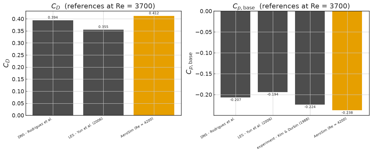
The subcritical turbulent sphere has well-established integral quantities at Re = 3700 (DNS, LES and experiment). The run is at Re = 4200; these quantities are nearly Re-flat across that range, so the comparison carries a ~13% Reynolds offset (see reference/REFERENCES.md). The drag is the total (direct IBM force) drag from the run and the base pressure is taken from the run’s surface pressure; the recirculation length and separation angle need the wake field and are shown as references only.

# Re=3700 integral-quantity benchmark (subcritical turbulent sphere) vs the
# Re=4200 run. The integral quantities are nearly Re-flat across this range, so
# the comparison carries a ~13% Re offset (see reference/REFERENCES.md).
df_int = pd.read_csv(
    "validation/external_aero/01_flow_over_sphere/reference/sphere_integral_Re3700.csv",
    comment="#",
)

# Run quantities at Re=4200: the total drag (direct IBM force, from force_stats)
# and the base pressure from the time-mean surface pressure.
hs = sim_turb.output.exports["default_series"].series.bodies["sphere"]
df_rho = hs.read_full_data("rho")
df_rho = df_rho[df_rho["time_step"] >= STATS_START].drop(columns="time_step")
cp_mean_nodes = (df_rho.mean().to_numpy() - RHO_INF) / (1.5 * RHO_INF * U_INF**2)
pts = pd.read_csv(hs.points_filename)
base_cp_run = float(cp_mean_nodes[pts["x"].to_numpy().argmax()])  # rearmost (base) node
run_vals = {"Cd": force_stats[4200]["Cd_mean"], "base_Cp": base_cp_run}

# Conventional-notation axis labels for each integral quantity.
q_labels = {"Cd": "$C_D$", "base_Cp": "$C_{p,\\mathrm{base}}$"}


def _short_ref(full: str) -> str:
    """Compact 'First-author et al. (year)' label from a full attribution string."""
    full = str(full).strip()
    year = ""
    if "(" in full and ")" in full:
        year = " " + full[full.index("(") : full.index(")") + 1]
        full = full[: full.index("(")].strip()
    surnames = [p.strip().split()[-1] for p in full.replace(" & ", ",").split(",") if p.strip()]
    if len(surnames) == 1:
        base = surnames[0]
    elif len(surnames) == 2:
        base = f"{surnames[0]} & {surnames[1]}"
    else:
        base = f"{surnames[0]} et al."
    return base + year


# The run only produces Cd and base_Cp from the surface data; recirculation length
# and separation angle need the wake field and are omitted here (references only).
# Each reference bar is labelled with its SOURCE (whose DNS/LES/experiment it is),
# read from the reference CSV's `reference` column - not a bare "DNS"/"LES".
fig_int, ax_int = common.fig_double()
for axq, q in zip(ax_int, ["Cd", "base_Cp"]):
    sub = df_int[df_int["quantity"] == q]
    labels = [f"{r.ref_type} - {_short_ref(r.reference)}" for r in sub.itertuples()]
    values = list(sub["value"])
    bar_colors = [common.colors.exp] * len(values)
    labels.append("AeroSim (Re = 4200)")
    values.append(run_vals[q])
    bar_colors.append(common.colors.sim)
    xq = np.arange(len(values))
    bars = axq.bar(xq, values, color=bar_colors)
    axq.bar_label(bars, fmt="%.3f", fontsize=8, padding=2)
    axq.axhline(0.0, color=common.colors.refline, lw=0.8)
    axq.set_xticks(xq)
    axq.set_xticklabels(labels, rotation=30, ha="right", fontsize=8)
    common.bar_axis(axq)
    axq.set_ylabel(q_labels[q])
    axq.set_title(f"{q_labels[q]}  (references at Re = 3700)")

plt.tight_layout()
plt.show(fig_int)

Vortex shedding and spectra

The lift-force power spectrum exposes the vortex-shedding peak. The low-mode Strouhal number plateaus near \(St \approx 0.19\) at high Reynolds number (Sakamoto & Haniu, 1990). The wake velocity probe gives an independent, velocity-based estimate of the same frequency.

from nassu.viz import energy_spectrum, read_series

# Low-mode shedding Strouhal reference (digitized Sakamoto & Haniu 1990 Fig. 7).
df_st = pd.read_csv(
    "validation/external_aero/01_flow_over_sphere/reference/sphere_strouhal.csv",
    comment="#",
)

fig, ax = common.fig_double()
for i, (scfg, Re, title) in enumerate(runs):
    s = force_stats[Re]
    cF, t, D = s["cF"], s["time"], s["D"]

    # The transverse (lift) force fluctuation carries the vortex-shedding signal.
    dt = float(np.median(np.diff(t)))
    f, S = energy_spectrum(cF[:, 2], dt)
    St = f * D / U_INF
    ax[i].loglog(St, S, color=common.colors.sim, alpha=0.8, label=r"$C_L$ (pressure force)")

    # Independent, velocity-based check: the wake velocity probe, a max-rate
    # instantaneous series export sampled every finest-level iteration (#1023);
    # time_step is in level-0 steps.
    try:
        probe = scfg.output.exports["spectrum"].series.points["point_velocity_wake"]
        dfw = read_series(probe, "ux", start_step=STATS_START)
        dtw = float(np.median(np.diff(dfw["time_step"])))
        ux_wake = dfw.drop(columns="time_step").iloc[:, 0].to_numpy()
        fw, Sw = energy_spectrum(ux_wake, dtw)
        ax[i].loglog(fw * D / U_INF, Sw, color=common.colors.exp, alpha=0.5, label=r"wake $u_x$")
    except (KeyError, AttributeError, FileNotFoundError, ValueError):
        pass

    # Reference low-mode Strouhal at this Re (interpolated off the digitized curve)
    # and the dominant peak of the lift spectrum.
    st_ref = float(np.interp(Re, df_st["Re"], df_st["St"]))
    st_peak = float(St[np.argmax(S)])
    ax[i].axvline(
        st_ref, color=common.colors.refline, ls="--", alpha=0.8, label=f"St ref = {st_ref:.2f}"
    )
    ax[i].axvline(
        st_peak, color=common.colors.sim, ls=":", alpha=0.8, label=f"St peak = {st_peak:.2f}"
    )

    ax[i].set_title(title)
    ax[i].set_xlabel(r"$St = f\,D/U$")
    ax[i].set_ylabel("PSD")
    ax[i].legend(fontsize="small")

plt.tight_layout()
plt.show(fig)

Flow field

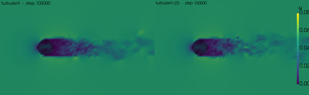
Instantaneous velocity magnitude on the lateral plane through the sphere centre (plane_series.mid_sphere): wake view for the turbulent runs, framed from the sphere geometry.

viz.enable_offscreen()

labels = {
    "turbulentFlowOverSphere": "turbulent",
    "turbulentFlowOverSphereLES": "turbulent LES",
}
cfg0 = sim_cfgs["turbulentFlowOverSphere", 0]
body, geom = viz.read_body(cfg0, "sphere")
view = viz.frame_body(geom, "y", slice_coord=64.0, downstream=2.0, half_extent=3.0)

panels = [
    viz.Panel(
        label,
        viz.PlaneSource.from_cfg(sim_cfgs[name, 0], series="plane_series", plane="mid_sphere"),
        view,
    )
    for name, label in labels.items()
]
steps = [panels[0].source.steps[-1]]
plotter = viz.render_grid(
    panels,
    steps=steps,
    scalar="u_mag",
    cmap="viridis",
    clim=(0.0, 0.08),
    bar_title="|u|",
    bodies=[body],
)
plotter.show()

/tmp/ipykernel_3072641/1996413703.py:29: UserWarning: Using static image for notebook display.
Install trame for interactive backends: pip install "pyvista[jupyter]"
  plotter.show()

Version

sim_info = sim_cfg.output.read_info()

nassu_commit = sim_info["commit"]
nassu_version = sim_info["version"]
print("Version:", nassu_version)
print("Commit hash:", nassu_commit)

Version: 2.0.0a1
Commit hash: a9e18ca8bb03b24ce4d631e70482ec8cf66e7cef

Configuration

from IPython.display import Code

Code(filename=filename)

simulations:
  - name: laminarFlowOverSphere
    save_path: ./validation/external_aero/01_flow_over_sphere/results/laminar

    n_steps: 40000

    report: {frequency: 1000}

    domain:
      domain_size:
        x: 480
        y: 160
        z: 160
      block_size: 8
      bodies:
        sphere:
          geometry_path: fixture/stl/basic/sphere.stl
          transformation:
            scale: [1.6, 1.6, 1.6]
            translation: [112, 72, 72]
      refinement:
        static:
          default:
            volumes_refine:
              - start: [96, 64, 64]
                end: [160, 96, 96]
                lvl: 1
                is_abs: true

    data:
      export_IBM_nodes:
        ibm_exp:
          body_name: sphere
          frequency: 5000
      body_nodes:
        # Per-source-triangle skin-friction primitives (issue #879): the friction
        # velocity `friction_u_tau` and `friction_y_plus`, plus the aggregated
        # viscous-traction vector and centroid/normal/area, written as a flat
        # CSV/HDF time series. `nassu.viz.friction` derives the form/friction drag
        # split from these (issue #876). Sampled late in the steady run. The
        # quantities are listed explicitly so the exported IBM wall values (y+,
        # u_tau, traction) are unambiguous.
        friction:
          body_name: sphere
          mode: triangle
          frequency: 5000
          quantities:
            - friction_u_tau
            - friction_y_plus
            - traction_x
            - traction_y
            - traction_z
            - area
            - rho_interp
      exports:
        default:
          macrs: [rho, u]
          interval:
            frequency: 10000
            lvl: 0
          target:
            volume: {}
          outputs:
            instantaneous: true
        # Surface-pressure history over the sphere nodes: the mechanical form
        # (pressure) drag is integrated from the mean surface `rho` (Cp), then
        # added to the viscous `body_nodes.friction` split for the full drag.
        # Named `default_series` so the analysis reads it through the same
        # accessor as the turbulent runs; the turbulent child fully overrides it.
        default_series:
          macrs: ["rho"]
          interval: {frequency: 1000, lvl: 0}
          target:
            bodies:
              sphere:
                body_name: sphere
                normal_offset: 0.25
          outputs:
            instantaneous: true
        plane_series:
          macrs: ["rho", "u"]
          interval: {frequency: 5000, lvl: 0}
          target:
            planes:
              # Lateral (y-normal) plane through the sphere centre: wake view.
              # Children override axis_pos for their own sphere position.
              mid_sphere:
                axis: y
                axis_pos: 80
                dist: 1

          outputs:
            instantaneous: true
    models:
      precision:
        default: single

      LBM:
        tau: 0.51
        vel_set: D3Q27
        coll_oper: RRBGK
      initialization:
        equations:
          rho: "1.0"
          ux: !unroll ["0.007854", "0.024583", "0.064583"]
          uy: "0"
          uz: "0"
      engine:
        name: CUDA

      BC:
        periodic_dims: [false, false, false]
        BC_map:
          - pos: N
            BC: Neumann
            wall_normal: N
            order: 0

          - pos: S
            BC: Neumann
            wall_normal: S
            order: 0

          - pos: F
            BC: Neumann
            wall_normal: F
            order: 1

          - pos: B
            BC: Neumann
            wall_normal: B
            order: 1

          - pos: E
            BC: RegularizedNeumannOutlet
            rho: 1.0
            wall_normal: E
            order: 2

          - pos: W
            BC: UniformFlow
            wall_normal: W
            rho: 1
            ux: !unroll [0.007854, 0.024583, 0.064583]
            uy: 0
            uz: 0
            order: 2

          - pos: NF
            BC: Neumann
            wall_normal: N
            order: 0

          - pos: NB
            BC: Neumann
            wall_normal: N
            order: 0

          - pos: SF
            BC: Neumann
            wall_normal: S
            order: 0

          - pos: SB
            BC: Neumann
            wall_normal: S
            order: 0

          - pos: NF
            BC: Neumann
            wall_normal: F
            order: 1

          - pos: NB
            BC: Neumann
            wall_normal: B
            order: 1

          - pos: SF
            BC: Neumann
            wall_normal: F
            order: 1

          - pos: SB
            BC: Neumann
            wall_normal: B
            order: 1

      IBM:
        forces_accomodate_time: 1000
        body_cfgs:
          default: {}

      multiblock:
        overlap_F2C: 2

  - name: turbulentFlowOverSphere
    parent: laminarFlowOverSphere

    save_path: ./validation/external_aero/01_flow_over_sphere/results/turbulent

    n_steps: 100000

    domain:
      domain_size:
        x: 640
        y: 128
        z: 128
      block_size: 8

      bodies: !not-inherit
        sphere:
          small_triangles: "add"
          geometry_path: fixture/stl/basic/sphere.stl
          transformation:
            scale: [0.8, 0.8, 0.8]
            translation: [112, 60, 60]

      refinement:
        static:
          default:
            volumes_refine:
              - start: [96, 32, 32]
                end: [224, 96, 96]
                lvl: 1
                is_abs: true
              - start: [104, 56, 56]
                end: [144, 72, 72]
                lvl: 3
                is_abs: true

    data:
      exports:
        default:
          interval: {frequency: 25000}
        default_series:
          macrs: ["u", "rho"]
          interval: {frequency: 20, lvl: 0}
          target:
            bodies:
              sphere:
                body_name: sphere
                normal_offset: 0.25
          outputs:
            instantaneous: true
        plane_series:
          interval: {frequency: 10000}
          target:
            planes:
              # Sphere centre for this domain size.
              mid_sphere: {axis_pos: 64}
        spectrum:
          macrs: ["rho", "u"]
          interval:
            frequency: 0
            lvl: 0
          target:
            points:
              # Centreline wake point ~2 diameters downstream of the sphere
              # centre (~(116, 64, 64), D~8), inside the lvl-3 refinement box:
              # independent velocity-based shedding-frequency (Strouhal) check.
              point_velocity_wake:
                pos: [132, 64, 64]
          outputs:
            spectrum: true

    models:
      LBM:
        tau: 0.500285714285714
        vel_set: D3Q27
        coll_oper: RRBGK
      initialization: !not-inherit
        rho: 1.0
        u:
          x: 0.05
          y: 0
          z: 0
      IBM:
        forces_accomodate_time: 5000
      multiblock:
        overlap_F2C: 2

      BC:
        periodic_dims: [false, false, false]
        BC_map:
          - pos: N
            BC: Neumann
            wall_normal: N
            order: 0

          - pos: S
            BC: Neumann
            wall_normal: S
            order: 0

          - pos: F
            BC: Neumann
            wall_normal: F
            order: 1

          - pos: B
            BC: Neumann
            wall_normal: B
            order: 1

          - pos: E
            BC: RegularizedNeumannOutlet
            rho: 1.0
            wall_normal: E
            order: 2

          - pos: W
            BC: UniformFlow
            wall_normal: W
            rho: 1
            ux: 0.05
            uy: 0
            uz: 0
            order: 2

  - name: turbulentFlowOverSphereLES
    parent: turbulentFlowOverSphere

    models:
      LBM:
        tau: 0.500024

      LES:
        model: Smagorinsky
        sgs_cte: 0.17