Boundary Conditions¶

Scalar boundary conditions in nassu follow the same regularised macroscopic-target style as the fluid BCs Latt et al.[1]: the user prescribes the macroscopic quantity at the wall (a scalar value, a flux, or a convective relation), and the populations $g_i$ are reconstructed from the prescribed macros.

The available BC types are listed below. A scalar BC imposes no velocity of its own; the advection velocity that enters the reconstruction is the local fluid velocity.

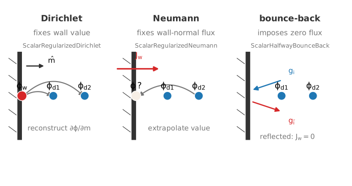
../../_images/scalar_bc_types.svg — The three scalar boundary-condition families. Dirichlet fixes the wall value $\phi_w$ and reconstructs the inward gradient; Neumann fixes the wall-normal flux $J_w$ and extrapolates the value; bounce-back reflects the populations to impose zero flux. Each infers the unknowns it does not prescribe from the interior nodes.¶

Applicability of the scalar wall conditions

A wall value (Dirichlet) applies to a fixed-temperature or fixed-concentration surface. A wall flux (Neumann) applies to a known heat or mass release, including the adiabatic case $J_w = 0$. A convective relation (Robin) applies to a wall losing heat to a far-field ambient through a transfer coefficient, as in naturally-ventilated compartment and room-fire problems. Bounce-back applies to an insulated or symmetry surface, imposing zero flux directly without an off-wall reference point.

Where each wall condition attaches¶

A scalar wall condition attaches to one of two geometry kinds: a Cartesian domain face, or a voxelized solid body (an STL rasterized onto the lattice, see Voxelization of Solid-Body Scalar Boundaries). The scalar boundary conditions are LBM-style only: there is no IBM-surface, wall-model, or SEM scalar wall variant. A solid body inside the domain is given a scalar wall by voxelizing it, which classifies the surface band and attaches the same regularised reconstructions to the band nodes.

The DDF scalar wall conditions and the variable-density energy-field temperature walls reach those kinds differently:

Wall condition	Domain faces	Voxelized solid body
DDF Dirichlet (`ScalarRegularizedDirichlet`)	yes	yes
DDF Neumann (`ScalarRegularizedNeumann`)	yes	yes
DDF Robin (`ScalarRegularizedRobin`)	yes	yes
DDF bounce-back (`ScalarHWBB`)	yes	yes
Energy-field temperature (`TempDirichlet` / `TempNeumann` / `TempRobin`)	yes (6 cardinal faces)	not available

The DDF scalar walls (ScalarHWBB, ScalarRegularizedDirichlet, ScalarRegularizedNeumann, ScalarRegularizedRobin) carry the Boussinesq scalar-temperature route and reach both domain faces and voxelized bodies. The energy-field temperature walls (TempDirichlet, TempNeumann, TempRobin) of the variable-density route attach to the six cardinal domain faces of the finite-difference energy field. A voxelized solid body in a variable-density thermal run carries an adiabatic wall (the TempNeumann zero-flux default).

Dirichlet - prescribed scalar value¶

ScalarRegularizedDirichlet enforces a prescribed scalar value $\phi_w$ at the wall.

The reconstruction at a wall node is:

Evaluate the equilibrium $g_i^{eq}$ from $(\phi_w, u)$ using the standard first-order equilibrium, where $u$ is the local fluid velocity (the scalar imposes no velocity of its own; the advection velocity comes from the fluid).
Estimate the inward gradient from the one-sided second-order finite difference along the inward unit normal $\hat{m}$ (with $\Delta x = 1$): $$\frac{\partial \phi}{\partial m} = \frac{-3\,\phi_w + 4\,\phi_{d1} - \phi_{d2}}{2},$$ where $\phi_{d1}$, $\phi_{d2}$ are the values one and two nodes into the fluid.
Set the stored non-equilibrium flux from the Chapman-Enskog rank-1 estimate, $q_\alpha^{neq} = -c_{s,\phi}^2\, \tau_g\, (\partial \phi / \partial m)\, m_\alpha$ (tangential components vanish; only the wall-normal gradient is estimated).
Reconstruct $g_i^{neq} = (w_i\, c_{i\alpha} / c_{s,\phi}^2)\, q_\alpha^{neq}$ and set $g_i = g_i^{eq} + g_i^{neq}$ at the wall node.

This mirrors the fluid RegularizedHalfwayBounceBack BC and reaches second-order accuracy in $\Delta x$ at the wall.

The advection velocity that enters the equilibrium is the local fluid velocity; the scalar BC prescribes only the wall value $\phi_w$ and does not impose a velocity.

Neumann - prescribed flux¶

ScalarRegularizedNeumann enforces a prescribed wall flux $J_w$. The convention used in nassu is:

$\hat{m}$ is the unit normal pointing from the wall into the fluid.
$J_w \equiv -D_{\text{total}}\, \partial \phi / \partial m$ is the prescribed flux, where $D_{\text{total}} = D_0 + D_{\text{SGS}}$ is the local total (molecular plus LES subgrid) diffusivity.
$J_w > 0$ corresponds to scalar flowing into the fluid; $J_w = 0$ is an adiabatic / zero-gradient boundary.

The reconstruction works on the stored moments. The wall value extrapolates the known-flux gradient through the one-sided second-order finite difference:

\[\phi = \frac{4\,\phi_{d1} - \phi_{d2} + 2\, J_w / D_{\text{total}}}{3}.\]

The stored non-equilibrium flux relates to the physical diffusive flux through the level-invariant form $J_\alpha = q_\alpha^{neq}\,(1 - \omega_\phi/2)$ (see the coupling page), and a positive influx points along $\hat{m}$, so the wall-normal component is

\[q_\alpha^{neq}\, m_\alpha = \frac{J_w}{1 - \omega_\phi/2},\]

combined with the tangential components inherited from the adjacent fluid node. The populations follow as $g_i = g_i^{eq} + g_i^{neq}$ at the boundary node.

Robin - convective wall heat loss¶

ScalarRegularizedRobin is the convective (mixed) wall: the wall flux is proportional to the difference between the local wall value and a far-field ambient,

\[J_w = h\,(\phi_\infty - \phi_w),\]

with $h$ the transfer coefficient and $\phi_\infty$ the ambient. It is the LBM-scalar analogue of the standard convective heat-loss wall used for naturally-ventilated compartment and room-fire problems. A wall hotter than ambient loses scalar ($J_w < 0$), in the same influx-positive convention as the Neumann wall.

The wall value is unknown and resolved on the fly. Combining the convective flux with the diffusive relation $\partial \phi / \partial m = -J_w / D_{\text{total}}$ and the one-sided second-order finite difference for the inward gradient gives a linear balance whose solution is

\[\phi_w = \frac{2\,h\,\phi_\infty / D_{\text{total}} + 4\,\phi_{d1} - \phi_{d2}}{3 + 2\,h / D_{\text{total}}},\]

where $D_{\text{total}} = D_0 + D_{\text{SGS}}$ is the LES-inclusive level diffusivity. The resolved flux $J_w = h\,(\phi_\infty - \phi_w)$ is then imposed through the same prescribed-flux reconstruction as the Neumann wall (the wall-normal stored flux $q_\alpha^{neq} m_\alpha = J_w / (1 - \omega_\phi/2)$ with tangential components inherited), so the convective wall reuses the validated flux path rather than a separate reconstruction.

The two limits are exact:

$h \to 0$ recovers the adiabatic Neumann zero-flux wall, $\phi_w \to (4\,\phi_{d1} - \phi_{d2})/3$ with $J_w \to 0$.
$h \to \infty$ recovers the Dirichlet wall at the ambient, $\phi_w \to \phi_\infty$.

The coefficient $h$ is supplied as a lattice velocity at level 0. A dimensional film coefficient $h_{\text{phys}}$ in W/m^2 K is converted through $h_{\text{lat}} = \left( h_{\text{phys}} / (\rho\,c_p) \right)\,\Delta t / \Delta x$, where the velocity scaling $\Delta t / \Delta x$ is the same factor applied to the inlet velocity.

Bounce-back - adiabatic wall¶

ScalarHalfwayBounceBack is the zero-flux (adiabatic / insulating) wall. The post-stream populations are reflected back along their incoming directions, so no scalar crosses the boundary and the wall-normal gradient vanishes. It is the scalar counterpart of the fluid HalfwayBounceBack and is the natural choice for insulated or symmetry surfaces where neither a value nor a non-zero flux is prescribed. The same condition is recovered as the $J_w = 0$ case of the Neumann reconstruction above; bounce-back imposes it directly, without an off-wall reference point. In the macroscopic-only storage the populations are rebuilt from the node’s post-collision moments before the reflection, exactly as the fluid bounce-back does. The regularised $J_w = 0$ Neumann form imposes the same zero-flux wall in strictly conservative form where an off-wall stencil exists.

Inlet profiles¶

Scalar values at the domain inlet are prescribed through the regularised Dirichlet form, with the inlet velocity taken from the fluid inlet BC (uniform-flow or SEM). A spatially varying $\phi_{\text{inlet}}(z)$ profile is supported through the symbolic configuration.