From the Lattice to Navier-Stokes

This page answers the question that every newcomer eventually asks: why does pushing populations around a lattice reproduce the Navier-Stokes equations at all? The connection is not assumed; it is derived. The tool is the Chapman-Enskog expansion, a systematic multiscale analysis that extracts the macroscopic behaviour hidden inside the lattice Boltzmann equation [1][2].

The derivation also delivers the single most useful result of the whole chapter: the relation between the relaxation frequency \(\omega\) and the fluid viscosity, (10). That relation is what lets you set a physical viscosity in a simulation, and it is re-used on the lattice units page.

The level here is guided: the full skeleton plus the algebra that carries physical meaning. Steps that are pure bookkeeping are summarized rather than written out term by term; for those, the standard reference is Krüger et al.[2].

The idea: separating the scales

A turbulent flow has features on wildly different scales. The molecular collisions that the BGK operator models happen on the relaxation time \(\tau\), which is minuscule. The flow structures we care about, gusts and recirculation zones, evolve far more slowly and over far larger distances. Chapman-Enskog exploits exactly this separation.

Introduce a single small bookkeeping parameter \(\epsilon\), physically the Knudsen number \(\mathrm{Kn} = \ell / L\) introduced in the kinetic primer: the ratio of the molecular scale to the macroscopic scale. Smallness of \(\epsilon\) is the mathematical statement that the flow is close to a continuum. The analysis then expands every quantity in powers of \(\epsilon\) and collects terms order by order. Each order turns out to govern physics on its own scale.

Note

The Knudsen number \(\mathrm{Kn} = \ell / L\) compares the molecular mean free path \(\ell\) (the average distance a molecule travels between collisions) to the macroscopic length \(L\) of the flow. A small \(\mathrm{Kn}\) means collisions are so frequent that the gas behaves as a smooth continuum, which is exactly the regime where the Navier-Stokes equations hold and the expansion below is justified.

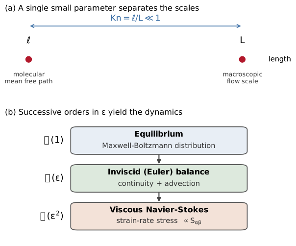
The single small parameter \(\epsilon = \mathrm{Kn}\) separates the molecular and macroscopic scales, and successive orders of the expansion yield first the inviscid (Euler) balance and then the viscous Navier-Stokes stress.

Step 1: expand the populations

The populations are written as the equilibrium plus a series of ever-smaller departures from it:

(1)\[ f_i = f_i^{(0)} + \epsilon f_i^{(1)} + \epsilon^2 f_i^{(2)} + \ldots \]

The leading term is the equilibrium itself, \(f_i^{(0)} = f_i^{\mathrm{eq}}\). This is forced by the physics of the kinetic primer: when collisions dominate (\(\epsilon \to 0\)), the distribution is Maxwell-Boltzmann. The higher terms \(f_i^{(1)}, f_i^{(2)}, \ldots\) are the successively smaller distortions that velocity gradients impress on it, and it is these distortions that will become the viscous stress.

The moment constraints fix what each correction is allowed to carry. By definition density and momentum are moments of \(f^{\mathrm{eq}}\) alone, so the corrections carry no mass and no momentum:

(2)\[ \sum_i f_i^{(n)} = 0, \qquad \sum_i f_i^{(n)} c_{i\alpha} = 0, \qquad n \geq 1 \]

These are the solvability conditions. They are not optional; they are what makes the expansion consistent, and they are used at every order below.

Step 2: expand the derivatives in time

Because slow flow structures and fast relaxation live on different time scales, a single time derivative is not enough. Chapman-Enskog splits it into a fast convective time and a slow diffusive time:

(3)\[ \partial_t = \epsilon\, \partial_t^{(1)} + \epsilon^2\, \partial_t^{(2)}, \qquad \partial_\alpha = \epsilon\, \partial_\alpha^{(1)} \]

The \(\partial_t^{(1)}\) scale carries inviscid (Euler) advection; the \(\partial_t^{(2)}\) scale carries the slower viscous diffusion. Space is rescaled once, since gradients are a single macroscopic-scale effect. This two-time-scale split is the heart of the method: it is why one kinetic equation can produce both the advective and the diffusive terms of Navier-Stokes [2].

Step 3: Taylor-expand the lattice equation

The lattice Boltzmann equation, (2), is exact in the sense that streaming is an exact shift. To compare it with differential equations we Taylor-expand the shifted populations about \((\boldsymbol{x}, t)\):

(4)\[ f_i(\boldsymbol{x} + \boldsymbol{c}_i \Delta t, t + \Delta t) = \sum_{n=0}^{\infty} \frac{\Delta t^n}{n!} \left(\partial_t + c_{i\alpha}\partial_\alpha\right)^n f_i \]

Keeping terms up to second order in \(\Delta t\) and substituting both the population expansion (1) and the time-scale split (3), the lattice equation separates, order by order in \(\epsilon\), into:

(5)\[ \mathcal{O}(\epsilon):\quad \left(\partial_t^{(1)} + c_{i\alpha}\partial_\alpha^{(1)}\right) f_i^{(0)} = -\frac{1}{\tau} f_i^{(1)} \]

(6)\[ \mathcal{O}(\epsilon^2):\quad \partial_t^{(2)} f_i^{(0)} + \left(\partial_t^{(1)} + c_{i\alpha}\partial_\alpha^{(1)}\right) \left(1 - \frac{\Delta t}{2\tau}\right) f_i^{(1)} = -\frac{1}{\tau} f_i^{(2)} \]

The factor \(\left(1 - \Delta t/(2\tau)\right)\) in (6) is not cosmetic. It is the fingerprint of the discrete second-order Taylor term, and it is precisely what shifts the bare relaxation time to its effective value. It is the reason the viscosity formula carries a \(-1/2\), as we are about to see.

Step 4: take moments and recover the equations

The macroscopic equations are obtained by summing the order-by-order equations over the discrete velocities, exactly as moments were taken in the kinetic primer.

Continuity. Summing (5) over \(i\), the right-hand side vanishes by the solvability condition (2), and the equilibrium moments give mass and momentum density. Adding the \(\mathcal{O}(\epsilon^2)\) mass equation and recombining the time scales yields the continuity equation exactly:

(7)\[ \partial_t \rho + \partial_\alpha(\rho u_\alpha) = 0 \]

Momentum. Multiplying (5) by \(c_{i\alpha}\) and summing gives the inviscid (Euler) momentum balance, in which the divergence of the equilibrium momentum flux appears,

(8)\[ \Pi_{\alpha\beta}^{(0)} = \sum_i f_i^{(0)} c_{i\alpha} c_{i\beta} = \rho u_\alpha u_\beta + \rho c_s^2\, \delta_{\alpha\beta} \]

The second term, \(\rho c_s^2 \delta_{\alpha\beta}\), is an isotropic pressure: the lattice Boltzmann method has an ideal-gas equation of state \(p = \rho c_s^2\). Pressure is not solved for separately; it is a moment of the equilibrium, just as the kinetic primer promised.

Viscous stress. The viscous term lives at \(\mathcal{O}(\epsilon^2)\) and comes from the first-order correction \(f_i^{(1)}\). Its second moment is the non-equilibrium stress \(\Pi_{\alpha\beta}^{(1)} = \sum_i f_i^{(1)} c_{i\alpha} c_{i\beta}\). Taking the second moment of (5) and using the equilibrium moments, the correction is proportional to the rate of strain [2]:

(9)\[ \Pi_{\alpha\beta}^{(1)} = -2\, \tau\, \rho c_s^2\, S_{\alpha\beta}, \qquad S_{\alpha\beta} = \frac{1}{2}\left(\partial_\alpha u_\beta + \partial_\beta u_\alpha\right) \]

This is the punchline of the whole construction. The departure of the populations from equilibrium is a strain-rate-proportional stress: that is exactly Newton’s law of viscosity, derived rather than postulated. It also connects directly to the solver: this \(\Pi_{\alpha\beta}^{(1)}\) is the \(\Pi_{\alpha\beta}^{\mathrm{neq}}\) that the moment-collision and LES routines read off the populations (see macroscopics).

Note

A Newtonian fluid is one whose viscous stress is directly proportional to the local rate of strain, with the viscosity as the constant of proportionality. Air and water are Newtonian to excellent approximation. Equation (9) shows that the lattice Boltzmann method reproduces exactly this linear stress-strain law, rather than imposing it.

Assembling the inviscid and viscous parts gives the momentum equation in the form already quoted on the macroscopics page, (1).

Step 5: read off the viscosity

Comparing the recovered momentum equation with the Navier-Stokes equation term by term identifies the kinematic viscosity. Carrying the discrete \(\left(1 - \Delta t/(2\tau)\right)\) factor of (6) through the algebra shifts \(\tau\) to its effective value, and the result is the central relation of the method [2]:

(10)\[ \nu = c_s^2 \left(\tau - \frac{\Delta t}{2}\right), \qquad\text{equivalently}\qquad \eta = \rho\, c_s^2\, \Delta t \left(\frac{1}{\omega} - \frac{1}{2}\right) \]

with \(\omega = \Delta t/\tau\) the relaxation frequency. The right-hand form is identical to (2) on the macroscopics page; the derivation here is where it comes from.

Two consequences are worth stating plainly:

• The \(-\Delta t/2\) is a discretization correction, not a continuum effect. It is the price of representing the streaming step exactly while comparing against differential equations, and it is what lets the lattice scheme reach second-order accuracy.

• Positivity of \(\nu\) requires \(\tau > \Delta t/2\), i.e. \(\omega < 2\). As \(\omega \to 2\) the viscosity goes to zero, which is the high-Reynolds-number limit. This is why the stability of the collision operator near \(\omega = 2\), the subject of the collision operators page, is what ultimately sets how high a Reynolds number the solver can reach.

Warning

The \(-\Delta t/2\) term is easy to drop, and dropping it silently corrupts the physics: it sets the viscosity wrong by a finite amount that no later step recovers. The relaxation time and the kinematic viscosity are tied by \(\nu = c_s^2(\tau - \Delta t/2)\), not \(\nu = c_s^2 \tau\).

Truncation error and the Ma < 0.1 constraint

The recovery above is not exact; it is correct only up to the order at which the expansion was truncated. Two distinct error families remain, and both bound how the method may be used.

Compressibility error. The lattice Boltzmann method is weakly compressible: its pressure follows the ideal-gas law \(p = \rho c_s^2\), so density is not held strictly constant. Density fluctuations scale with the square of the Mach number, \(\delta\rho/\rho \sim \mathrm{Ma}^2\), where \(\mathrm{Ma} = u/c_s\). To approximate incompressible flows faithfully, these spurious density variations must be kept small, which forces a low Mach number [2].

Higher-order truncation error. The standard equilibrium is itself a truncated Hermite expansion (see the collision operators page). The first neglected term introduces an \(\mathcal{O}(\mathrm{Ma}^3)\) error in the recovered momentum flux. This is a second, independent reason to keep the Mach number low.

Both errors shrink as \(\mathrm{Ma}\) decreases, and in practice a working threshold is \(\mathrm{Ma} < 0.1\), where the density fluctuations and the truncation error are both at or below the percent level [2]. This is the origin of the Mach-number constraint used throughout the solver, and the practical recipe for staying below it (by choosing the lattice velocity) is on the lattice units page.

Weak compressibility and acoustics

The weak compressibility just described is normally treated as an error to be minimized, but it has a constructive flip side that is worth keeping in view. Because the pressure follows \(p = \rho c_s^2\) with a finite speed of sound \(c_s\), a pressure disturbance in the lattice Boltzmann method does not equilibrate instantaneously the way it does in a strictly incompressible solver, where pressure is fixed by an elliptic Poisson equation. Instead it propagates as a genuine acoustic wave travelling at \(c_s\). The method carries sound as part of its native dynamics, with no separate acoustic model and no extra equation to solve [2].

This points to an application beyond mean and fluctuating loads: aeroacoustics, the prediction of flow-generated noise. Vehicle and pantograph noise, the aeroacoustics of ventilation and HVAC ducts, and wind noise around buildings, balconies and louvres are all problems where the sound is radiated by the same turbulent flow the solver already resolves. Because the lattice Boltzmann method resolves the acoustic field directly, it can in principle predict this noise without layering an acoustic analogy (such as Lighthill’s) on top of an incompressible solution [3].

Direct noise computation is demanding: the acoustic fluctuations are orders of magnitude weaker than the hydrodynamic ones, so it requires very low numerical dissipation, careful control of the Mach number, and non-reflecting boundary conditions at the domain edges [3]. The low-dissipation regularized RR-BGK operator that Nassu uses is well suited to this regime, the same weak compressibility that bounds the incompressible accuracy here being precisely what carries the acoustic field. Nassu does not currently target aeroacoustics as a validated capability.

What this recovers, and where it holds

The Chapman-Enskog analysis is the contract between the mesoscopic and the macroscopic descriptions. It guarantees that, in the low-Knudsen and low-Mach regime targeted here, streaming and colliding populations on a lattice solves the incompressible Navier-Stokes equations to second-order accuracy, with a viscosity you control through \(\omega\). Outside that regime, at high Knudsen or high Mach, the recovery degrades and the heavier compressible formulation is needed.

Next steps

The next page revisits the macroscopic quantities \(\rho\), \(u_\alpha\), \(\Pi_{\alpha\beta}^{\mathrm{neq}}\) and \(S_{\alpha\beta}\) that this derivation produced, and gives their discrete moment definitions as used by the solver.

---

[1]

Sydney Chapman and TG Cowling. The mathematical theory of non uniform gases, cambridge mathematical library. 1970.

[2] (1,2,3,4,5,6,7,8)

Timm Krüger, Halim Kusumaatmaja, Alexandr Kuzmin, Orest Shardt, Goncalo Silva, and Erlend Magnus Viggen. The lattice Boltzmann method. Graduate Texts in Physics. Springer International Publishing, Basel, Switzerland, 1 edition, November 2016.

[3] (1,2)

Simon Marié, Denis Ricot, and Pierre Sagaut. Comparison between lattice Boltzmann method and Navier-Stokes high order schemes for computational aeroacoustics. Journal of Computational Physics, 228(4):1056–1070, 2009. doi:10.1016/j.jcp.2008.10.021.