
 AeroSim Docs
Case 14 - Differentially heated square cavity (de Vahl Davis 1983)
Validation of the scalar-transport Boussinesq buoyancy path against the classic de Vahl Davis (1983) natural-convection benchmark.
A square cavity (side \(L = 128\)) has two opposing vertical walls held at fixed scalar values - hot west (\(\phi = 1\)) and cold east (\(\phi = 0\)) - and two adiabatic horizontal walls. The scalar temperature couples back onto the fluid through the Boussinesq body force
with gravity along \(-y\), so a hot parcel (\(\phi > \phi_\text{ref}\)) feels an upward force. The resulting buoyant recirculation is compared to the benchmark across three Rayleigh numbers.
Ra / Pr mapping
Fixing the buoyant velocity scale \(U = \sqrt{g\,\beta\,\Delta T\,L}\) and the cavity side \(L\) (with \(\Delta T = 1\), \(\text{Pr} = 0.71\)):
\(\beta = U^2/(\Delta T\,L)\) is identical for all three runs; only \(\nu\) (fluid \(\tau\)) and \(D\) (scalar diffusivity) change with Ra. The thermal diffusivity \(\alpha = D\) is used to nondimensionalise the velocities (\(u^\* = u\,L/\alpha\)).
Acceptance criteria
Against comparison/Differentially_heated_cavity/de_vahl_davis_1983.csv:
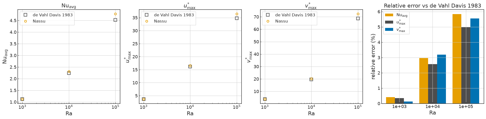
Nu_avg (hot-wall average Nusselt number) within 3% for all Ra.
Velocity extrema (\(u_\max\), \(v_\max\)) within 5%.
Reference: de Vahl Davis, G. (1983). Natural convection of air in a square cavity: a bench-mark numerical solution. Int. J. Numer. Methods Fluids 3(3):249-264.
[1]:
import pathlib

import matplotlib.pyplot as plt
import numpy as np
import pandas as pd
import pyvista as pv

import nassu.viz as common
from nassu.cfg.model import ConfigScheme

common.use_style()
pv.OFF_SCREEN = True
[2]:
def _find_project_root() -> pathlib.Path:
    here = pathlib.Path.cwd().resolve()
    for cand in [here, *here.parents]:
        if (cand / "pyproject.toml").exists() and (cand / "nassu").is_dir():
            return cand
    raise RuntimeError(f"Could not locate Nassu project root upward from {here}")


project_root = _find_project_root()
case_path = (
    project_root
    / "validation/thermal/01_differentially_heated_cavity/01_differentially_heated_cavity.nassu.yaml"
)
comparison_csv = (
    project_root
    / "validation/thermal/01_differentially_heated_cavity/reference/de_vahl_davis_1983.csv"
)

# Cavity geometry (lattice units), shared by all three Ra runs.
L = 128.0
DT = 1.0  # hot - cold scalar difference

# The three Ra variants are unrolled from one block; key them by Ra using the
# unroll order (1e3, 1e4, 1e5) so the labels line up with the benchmark table.
RA_BY_SIM_ID = {0: 1e3, 1: 1e4, 2: 1e5}

all_cfgs = ConfigScheme.sim_cfgs_from_file_dct(str(case_path))

sims = {}
for (name, sim_id), cfg in all_cfgs.items():
    ra = RA_BY_SIM_ID[sim_id]
    scalar = cfg.models.scalar_transports["temperature"]
    diffusivity = float(scalar.adv_diff_equation.D)  # alpha = D (Pr = nu / D)
    xdmf_path = pathlib.Path(cfg.output.exports["default"].volumes["default"].inst.xdmf_filename)
    if not xdmf_path.is_absolute():
        xdmf_path = (project_root / xdmf_path).resolve()
    if not xdmf_path.exists():
        raise FileNotFoundError(
            f"No instantaneous XDMF for Ra={ra:.0e} (#{sim_id}) at {xdmf_path}.\n"
            "Run the case on GPU first: `uv run nassu run "
            "validation/thermal/01_differentially_heated_cavity/01_differentially_heated_cavity.nassu.yaml`"
        )
    reader = pv.get_reader(str(xdmf_path))
    sims[ra] = {"cfg": cfg, "reader": reader, "D": diffusivity}
    print(f"Ra={ra:.0e} (#{sim_id}): D={diffusivity:.5f}, xdmf={xdmf_path.name}")

ra_values = sorted(sims.keys())
Ra=1e+03 (#0): D=0.48038, xdmf=default.volume.default.inst.xdmf
Ra=1e+04 (#1): D=0.15191, xdmf=default.volume.default.inst.xdmf
Ra=1e+05 (#2): D=0.04804, xdmf=default.volume.default.inst.xdmf
Load the steady-state field
Each run exports a handful of late-time snapshots; we take the last one as the steady state. The Nassu XDMF is a block-structured MultiBlock of cell-centred macros, so we combine the blocks and read the exact cell-centre values straight onto the regular \(128\times128\) lattice at the cavity mid-span (\(z\) midpoint). Reading the cells directly (rather than interpolating through a point-data probe) preserves the steep near-wall scalar gradient that sets the hot-wall Nusselt
number.
[3]:
def load_steady_grid(reader: pv.BaseReader, n: int = 128) -> dict[str, np.ndarray]:
    """Read the last exported step onto an (n x n) cell-centred grid at mid-span.

    The Nassu XDMF is a block-structured ``MultiBlock`` of cell-centred macros.
    We combine the blocks and read the exact cell-centre values onto the regular
    (n x n) lattice at the central z layer - no interpolation, so the steep
    near-wall scalar gradient that sets the Nusselt number is preserved. (An
    earlier ``cell_data_to_point_data().sample()`` round trip smeared that
    gradient and biased Nu low by ~35%.)

    Returns a dict of (n, n) arrays indexed [iy, ix] for phi, ux, uy plus the
    1-D cell-centre coordinate arrays xs, ys (both in [0, L]).
    """
    reader.set_active_time_value(max(reader.time_values))
    grid = reader.read().combine()
    centres = np.asarray(grid.cell_centers().points)

    # Mid-span z layer (thin periodic slab): pick the central cell layer.
    z_layers = np.unique(centres[:, 2])
    in_layer = centres[:, 2] == z_layers[len(z_layers) // 2]

    # Cell centres sit at (i + 0.5); map straight to integer lattice indices.
    ix = np.rint(centres[:, 0] - 0.5).astype(int)
    iy = np.rint(centres[:, 1] - 0.5).astype(int)

    out = {"xs": np.arange(n) + 0.5, "ys": np.arange(n) + 0.5}
    for key in ("temperature_phi", "ux", "uy"):
        field = np.full((n, n), np.nan)
        values = np.asarray(grid.cell_data[key], dtype=float)
        field[iy[in_layer], ix[in_layer]] = values[in_layer]  # [iy, ix]
        if np.isnan(field).any():
            raise ValueError(f"Missing {key} cells when mapping onto the {n}x{n} grid")
        out[key] = field
    return out


for ra in ra_values:
    sims[ra]["grid"] = load_steady_grid(sims[ra]["reader"], n=int(L))
    print(f"Ra={ra:.0e}: loaded {int(L)}x{int(L)} steady grid")
Ra=1e+03: loaded 128x128 steady grid
Ra=1e+04: loaded 128x128 steady grid
Ra=1e+05: loaded 128x128 steady grid
Diagnostics
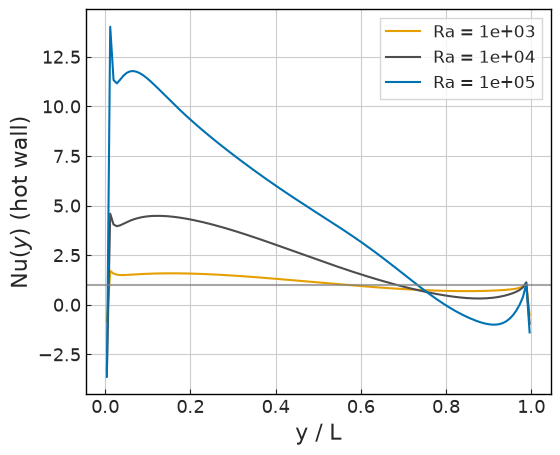
Hot-wall Nusselt number: \(\text{Nu}(y) = \dfrac{L}{\Delta T}\left.\dfrac{\partial\phi}{\partial x}\right|_{x=0}\), normalised so pure conduction gives \(\text{Nu} = 1\). The local wall gradient is estimated with a one-sided second-order difference from the first three cell columns; \(\text{Nu}_\text{avg}\) is its average over the wall height.
Velocity extrema: \(u_\max\) on the vertical mid-plane (\(x = L/2\)) and \(v_\max\) on the horizontal mid-plane (\(y = L/2\)), nondimensionalised by \(\alpha/L = D/L\) (\(u^\* = u_\text{lattice}\,L/D\)), with their locations normalised by \(L\).
[4]:
def hot_wall_nusselt(grid: dict[str, np.ndarray]) -> tuple[np.ndarray, np.ndarray, float]:
    """Local Nu(y) at the hot (west, x=0) wall and the height-averaged Nu_avg.

    The local wall-normal gradient d(phi)/dx is approximated with a one-sided
    2nd-order stencil on the first three cell columns, whose centres sit at
    x = 0.5, 1.5, 2.5 (spacing dx = 1 lattice unit):
        dphi/dx ~ (-3 phi0 + 4 phi1 - phi2) / (2 dx)
    The flux runs hot -> cold so dphi/dx < 0; Nu = -(L / dT) * dphi/dx flips the
    sign and normalises pure conduction (dphi/dx = -dT/L) to Nu = 1.
    """
    phi = grid["temperature_phi"]  # [iy, ix]
    ys = grid["ys"]
    dx = 1.0
    dphidx = (-3.0 * phi[:, 0] + 4.0 * phi[:, 1] - phi[:, 2]) / (2.0 * dx)
    nu_local = -(L / DT) * dphidx
    nu_avg = float(np.trapezoid(nu_local, ys) / (ys[-1] - ys[0]))
    return ys, nu_local, nu_avg


def velocity_extrema(grid: dict[str, np.ndarray], diffusivity: float) -> dict[str, float]:
    """u_max on the vertical mid-plane and v_max on the horizontal mid-plane.

    Velocities are nondimensionalised by alpha / L = D / L (u* = u * L / D).
    Locations are normalised by L.
    """
    ux = grid["ux"]  # horizontal velocity, [iy, ix]
    uy = grid["uy"]  # vertical velocity
    xs, ys = grid["xs"], grid["ys"]
    scale = L / diffusivity  # alpha = D

    # Vertical mid-plane x = L/2: profile of ux along y.
    ix_mid = int(L // 2)
    ux_col = ux[:, ix_mid]
    iy_u = int(np.argmax(np.abs(ux_col)))
    u_max = ux_col[iy_u] * scale
    y_umax = ys[iy_u] / L

    # Horizontal mid-plane y = L/2: profile of uy along x.
    iy_mid = int(L // 2)
    uy_row = uy[iy_mid, :]
    ix_v = int(np.argmax(np.abs(uy_row)))
    v_max = uy_row[ix_v] * scale
    x_vmax = xs[ix_v] / L

    return {
        "u_max": float(abs(u_max)),
        "y_umax": float(y_umax),
        "v_max": float(abs(v_max)),
        "x_vmax": float(x_vmax),
    }


for ra in ra_values:
    grid = sims[ra]["grid"]
    ys, nu_local, nu_avg = hot_wall_nusselt(grid)
    extrema = velocity_extrema(grid, sims[ra]["D"])
    sims[ra]["nu_y"] = (ys / L, nu_local)
    sims[ra]["metrics"] = {"Nu_avg": nu_avg, **extrema}
    print(f"Ra={ra:.0e}: ", {k: round(v, 4) for k, v in sims[ra]["metrics"].items()})
Ra=1e+03:  {'Nu_avg': 1.1167, 'u_max': 3.6386, 'y_umax': 0.1914, 'v_max': 3.6942, 'x_vmax': 0.1836}
Ra=1e+04:  {'Nu_avg': 2.2821, 'u_max': 16.7337, 'y_umax': 0.8242, 'v_max': 20.4119, 'x_vmax': 0.1211}
Ra=1e+05:  {'Nu_avg': 4.6864, 'u_max': 36.6986, 'y_umax': 0.8477, 'v_max': 72.8012, 'x_vmax': 0.0664}
Comparison table
Computed vs de Vahl Davis (1983) with relative error, and the tolerance assertions.
[5]:
ref = pd.read_csv(comparison_csv, comment="#")
ref = ref.set_index("Ra")

CMP = ["Nu_avg", "u_max", "v_max"]

rows = []
failures = []
for ra in ra_values:
    m = sims[ra]["metrics"]
    ref_row = ref.loc[float(ra)]
    for key in CMP:
        computed = m[key]
        reference = float(ref_row[key])
        rel_err = abs(computed - reference) / abs(reference)
        rows.append(
            {
                "Ra": f"{ra:.0e}",
                "quantity": key,
                "computed": computed,
                "reference": reference,
                "rel_err": rel_err,
            }
        )

table = pd.DataFrame(rows)
with pd.option_context("display.float_format", lambda v: f"{v:.4f}"):
    print(table.to_string(index=False))
   Ra quantity  computed  reference  rel_err
1e+03   Nu_avg    1.1167     1.1180   0.0012
1e+03    u_max    3.6386     3.6490   0.0029
1e+03    v_max    3.6942     3.6970   0.0008
1e+04   Nu_avg    2.2821     2.2430   0.0174
1e+04    u_max   16.7337    16.1780   0.0344
1e+04    v_max   20.4119    19.6170   0.0405
1e+05   Nu_avg    4.6864     4.5190   0.0371
1e+05    u_max   36.6986    34.7300   0.0567
1e+05    v_max   72.8012    68.5900   0.0614
Comparison plots
The table above, visualised. The left panels overlay the computed metric on the de Vahl Davis (1983) reference across Ra (one panel per quantity, log-x in Ra); the right panel shows the relative error of each metric across Ra.
[6]:
labels = {"Nu_avg": r"$\mathrm{Nu}_\mathrm{avg}$", "u_max": r"$u_\max^*$", "v_max": r"$v_\max^*$"}
ra_arr = np.array([float(ra) for ra in ra_values])

fig, axes = plt.subplots(1, len(CMP) + 1, figsize=(5 * (len(CMP) + 1), 5))

# One panel per quantity: computed vs de Vahl Davis reference across Ra.
for ax, key in zip(axes[:-1], CMP):
    computed = np.array([sims[ra]["metrics"][key] for ra in ra_values])
    reference = np.array([float(ref.loc[ra][key]) for ra in ra_values])
    ax.plot(ra_arr, reference, label="de Vahl Davis 1983", **common.markers.exp("s", markersize=9))
    ax.plot(ra_arr, computed, label="Nassu", **common.markers.sim("o"))
    ax.set_xscale("log")
    ax.set_xlabel("Ra")
    ax.set_ylabel(labels[key])
    ax.set_title(labels[key])
    ax.legend()

# Relative error of every metric across Ra.
ax = axes[-1]
width = 0.8 / len(CMP)
x = np.arange(len(ra_values))
for i, key in enumerate(CMP):
    rel_err = np.array(
        [
            abs(sims[ra]["metrics"][key] - float(ref.loc[ra][key])) / abs(float(ref.loc[ra][key]))
            for ra in ra_values
        ]
    )
    ax.bar(x + (i - (len(CMP) - 1) / 2) * width, 100 * rel_err, width, label=labels[key])
ax.set_xticks(x)
ax.set_xticklabels([f"{ra:.0e}" for ra in ra_values])
ax.set_xlabel("Ra")
ax.set_ylabel("relative error (%)")
ax.set_title("Relative error vs de Vahl Davis 1983")
ax.legend()

fig.tight_layout()
plt.show()
Isotherms and streamlines
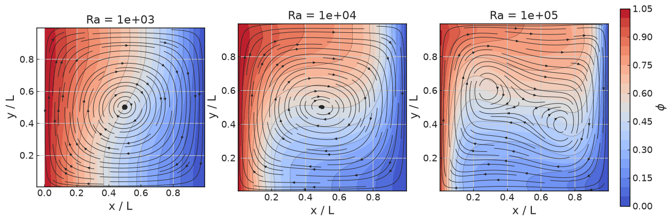
Steady scalar field (isotherms) with the buoyant recirculation overlaid as streamlines, one panel per Ra. The recirculation tightens and the thermal boundary layers thin as Ra increases.
[7]:
import matplotlib.pyplot as plt

fig, axes = plt.subplots(1, len(ra_values), figsize=(5 * len(ra_values), 5))
if len(ra_values) == 1:
    axes = [axes]

for ax, ra in zip(axes, ra_values):
    grid = sims[ra]["grid"]
    xs, ys = grid["xs"], grid["ys"]
    X, Y = np.meshgrid(xs / L, ys / L)
    phi = grid["temperature_phi"]
    cf = ax.contourf(X, Y, phi, levels=21, cmap="coolwarm")
    ax.contour(X, Y, phi, levels=11, colors="k", linewidths=0.4, alpha=0.5)
    ax.streamplot(
        xs / L,
        ys / L,
        grid["ux"],
        grid["uy"],
        color=common.colors.text,
        density=1.1,
        linewidth=0.7,
        arrowsize=0.7,
    )
    ax.set_title(f"Ra = {ra:.0e}")
    ax.set_xlabel("x / L")
    ax.set_ylabel("y / L")
    ax.set_aspect("equal")

fig.colorbar(cf, ax=axes, label=r"$\phi$", fraction=0.025, pad=0.02)
plt.show()
Local hot-wall Nusselt profile
\(\text{Nu}(y)\) along the hot (west) wall for each Ra. The peak near the bottom (where cold fluid impinges) sharpens with Ra; the height-averaged value is the \(\text{Nu}_\text{avg}\) compared above.
[8]:
fig, ax = common.fig_single()
shapes = common.markers.shapes()
for i, ra in enumerate(ra_values):
    y_norm, nu_local = sims[ra]["nu_y"]
    ax.plot(y_norm, nu_local, label=f"Ra = {ra:.0e}", linewidth=1.5)
common.refline(ax, 1.0)
ax.set_xlabel("y / L")
ax.set_ylabel(r"$\mathrm{Nu}(y)$ (hot wall)")
ax.legend()
plt.show()
Version
[9]:
sim_cfg = next(iter(ConfigScheme.sim_cfgs_from_file_dct(str(case_path)).values()))
sim_info = sim_cfg.output.read_info()

nassu_commit = sim_info["commit"]
nassu_version = sim_info["version"]
print("Version:", nassu_version)
print("Commit hash:", nassu_commit)
Version: 2.0.0a7
Commit hash: 5e47f2762575c2d285254d36bfd354b6af09fda1
Configuration
[10]:
from IPython.display import Code

Code(filename=str(case_path))
[10]:
# Differentially heated square cavity - de Vahl Davis (1983) benchmark
#
# Natural-convection benchmark for the scalar-transport Boussinesq
# buoyancy path. A square cavity with two opposing vertical walls held
# at fixed scalar values (hot W = 1, cold E = 0) and two adiabatic
# horizontal walls (N, S) develops a buoyancy-driven recirculation. The
# scalar `temperature` couples back onto the fluid through the Boussinesq
# body force F = -rho0 * beta * (phi - phi_ref) * gravity.
#
# This case validates the buoyancy coupling using only domain-face BCs
# (no voxelization / IBM needed).
#
# Quasi-2D: a thin slab in z (8 cells, periodic) reproduces the 2-D
# benchmark while staying on the 3-D D3Q27 fluid / D3Q7 scalar kernels
# (same pattern as case 12.2).
#
# ---------------------------------------------------------------------
# Non-dimensional mapping (Pr = 0.71, dT = 1, L = 128, U = 0.1)
# ---------------------------------------------------------------------
# The governing dimensionless groups are
#
#     Ra = g * beta * dT * L^3 / (nu * D)        (Rayleigh number)
#     Pr = nu / D                                (Prandtl number)
#
# We fix the buoyant velocity scale U = sqrt(g * beta * dT * L) and the
# cavity side L; then
#
#     nu   = U * L * sqrt(Pr / Ra)
#     D    = nu / Pr
#     beta = U^2 / (dT * L)            (with dT = 1)
#
# So fixing U and L fixes beta and the buoyancy force for ALL Ra; only
# nu (fluid tau) and D (scalar diffusivity) change with Ra. The implied
# gravity magnitude is g = U^2 / (beta * dT * L) = 1 (lattice), and the
# alpha used to nondimensionalise the benchmark velocities is alpha = D
# (Pr = nu/alpha = nu/D = 0.71 by construction).
#
# Fluid relaxation (cs^2 = 1/3): tau = nu / cs^2 + 1/2 = 3*nu + 1/2.
# Scalar relaxation (D3Q7, cs_phi^2 = 1/4): tau_phi = D / 0.25 + 1/2.
#
#   | Ra   | nu        | tau (fluid) | D         | tau_phi (D/0.25+0.5) |
#   | 1e3  | 0.341066  | 1.5232      | 0.480384  | 2.4215               |
#   | 1e4  | 0.107855  | 0.8236      | 0.151909  | 1.1076               |
#   | 1e5  | 0.034107  | 0.6023      | 0.048038  | 0.6922               |
#
# The tabulated fluid `tau` and scalar `D` below use the rounded values
# (tau = 1.5232 / 0.8236 / 0.6023; D = 0.48038 / 0.15191 / 0.04804).
# beta = U^2 / L = 0.1^2 / 128 = 7.8125e-5, identical for all three runs.
# Raising U from 0.04 to 0.1 scales nu and D up by 2.5x, cutting the
# step count to steady state by 2.5x while keeping Ra, Pr fixed; the peak
# Mach number stays <= 0.045 (well within the Ma < 0.1 limit).
#
# ---------------------------------------------------------------------
# Steady state and timing
# ---------------------------------------------------------------------
# Convective time scale L/U = 1280 steps; diffusive time scale L^2/D
# ranges from ~34k (Ra=1e3) to ~340k (Ra=1e5). The runs are seeded with
# a linear hot->cold horizontal ramp for the scalar to cut the transient.
# n_steps below is a generous fixed budget per Ra; it may be shortened
# using the `data.divergence` and `report` output once the wall Nusselt
# number and velocity extrema stop drifting.
#
# Reference: de Vahl Davis, G. (1983). "Natural convection of air in a
# square cavity: a bench-mark numerical solution." Int. J. Numer.
# Methods Fluids 3(3):249-264. Comparison data in
# validation/thermal/01_differentially_heated_cavity/reference/.

simulations:
  - name: differentiallyHeatedCavity
    save_path: !unroll
      - ./validation/thermal/01_differentially_heated_cavity/results/dvd_ra1e3
      - ./validation/thermal/01_differentially_heated_cavity/results/dvd_ra1e4
      - ./validation/thermal/01_differentially_heated_cavity/results/dvd_ra1e5
    n_steps: !unroll [240000, 200000, 200000]

    report:
      frequency: 2000

    domain:
      # Square cavity 128 x 128 in the x-y plane; thin periodic slab in z.
      domain_size:
        x: 128
        y: 128
        z: 8
      block_size: 8

    data:
      # Steady-state monitor: watch this flatten to size n_steps.
      exports:
        default:
          macrs: [rho, u, temperature_phi]
          interval:
            start_step: !unroll [216000, 180000, 180000]
            frequency: !unroll [8000, 10000, 10000]
            lvl: 0
          target:
            volumes:
              default: {}
          outputs:
            instantaneous: true
        plane_series:
          macrs: [u, temperature_phi]
          interval: {frequency: !unroll [8000, 10000, 10000], lvl: 0}
          target:
            planes:
              # Vertical mid-plane (x = L/2): u_y profile -> v_max location.
              vertical_mid:
                axis: x
                axis_pos: 64
                dist: 1
              # Horizontal mid-plane (y = L/2): u_x profile -> u_max location.
              horizontal_mid:
                axis: y
                axis_pos: 64
                dist: 1
              # slice full (z = L/2)
              slice_mid:
                axis: z
                axis_pos: 4
                dist: 1
          outputs:
            instantaneous: true

    models:
      precision:
        default: single

      LBM:
        # Fluid kinematic viscosity per Ra (Pr = 0.71, U = 0.1, L = 128).
        tau: !unroll [1.5232, 0.8236, 0.6023]
        vel_set: D3Q27
        coll_oper: HRRBGK

      LES:
        model: Smagorinsky
        sgs_cte: 0.1

      engine:
        name: CUDA

      # All four in-plane walls are no-slip (RegularizedHWBB). z is periodic.
      # x walls (W, E) carry the hot / cold scalar Dirichlet; y walls
      # (N, S) are adiabatic for the scalar (zero-flux bounce-back).
      BC:
        periodic_dims: [false, false, true]
        BC_map:
          - pos: W
            BC: RegularizedHWBB
            wall_normal: W
            order: 0
          - pos: E
            BC: RegularizedHWBB
            wall_normal: E
            order: 0
          - pos: N
            BC: RegularizedHWBB
            wall_normal: N
            order: 1
          - pos: S
            BC: RegularizedHWBB
            wall_normal: S
            order: 1

      scalar_transports:
        temperature:
          velocity_set: D3Q7
          collision_operator: RRBGK
          adv_diff_equation:
            # Scalar diffusivity per Ra (D = nu / Pr).
            D: !unroll [0.48038, 0.15191, 0.04804]
            S: "0"
          # Boussinesq coupling onto the fluid. beta = U^2 / L = 7.8125e-5,
          # gravity along -y (y is vertical); a hot parcel (phi > phi_ref)
          # then feels +y upward force via F = -rho0*beta*(phi-phi_ref)*g.
          buoyancy:
            beta: 7.8125e-5
            phi_ref: 0.5
            gravity: [0.0, -1.0, 0.0]
            rho0: 1.0
          # Linear hot->cold horizontal ramp (x is the lattice index,
          # 0..127). Seeds the scalar near its eventual conduction profile
          # to shorten the transient.
          initial_field: "1.0 - x / 127.0"
          BC:
            BC_map:
              # Hot vertical wall (west), phi = 1, no-slip.
              - pos: W
                BC: ScalarRegularizedDirichlet
                wall_normal: W
                params:
                  phi_w: 1.0
              - pos: E
                BC: ScalarRegularizedDirichlet
                wall_normal: E
                params:
                  phi_w: 0.0
              - pos: N
                BC: ScalarRegularizedNeumann
                params:
                  J_w: 0.0
                wall_normal: N
              - pos: S
                BC: ScalarRegularizedNeumann
                params:
                  J_w: 0.0
                wall_normal: S