Solid Wall

Solid wall boundary conditions are those which impose no-slip at a wall. The rate-of-strain can be either calculated from a finite difference scheme or a wall model.

Halfway Bounce-Back

For the halfway bounce-back (HWBB) the unknown populations are obtained by reflecting back the opposite post-collision populations.

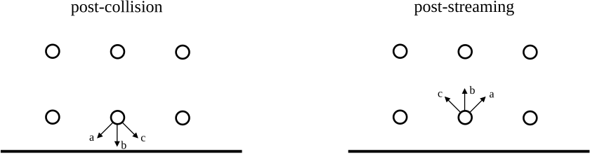
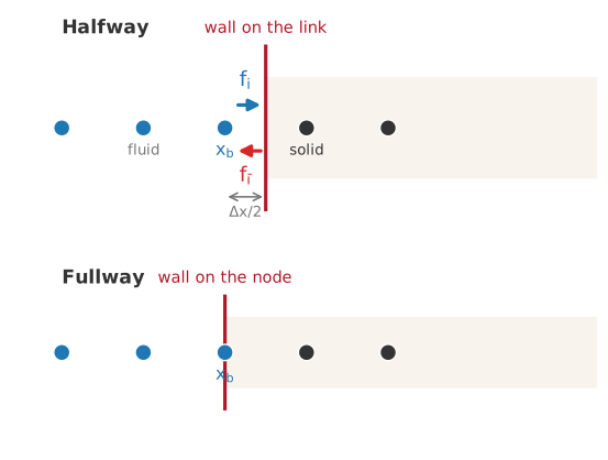
Halfway bounce-back. The wall lies on the link midway between the last fluid node and the first solid node; a population streaming into the wall is reflected back along the opposite direction after the stream. The wall therefore sits half a lattice spacing beyond the boundary node, unlike a fullway scheme where it coincides with the node.

Therefore, with the halfway bounce-back boundary condition, the unknown populations at streaming are given by:

(1)\[ f_{\bar{i}}\left(t+\Delta t\right)=f_{i}^{*}\left(t\right) \]

where \(\bar{i}\) is the opposite \(i\)-direction.

Use case

Halfway bounce-back represents a no-slip solid wall. Being fully local, it reads only the node’s own post-collision populations, which makes it cheap and simple to apply.

Note

The reflection places the wall on the link, halfway between the boundary node and its neighbor, so the wall does not coincide with a lattice node. The effective wall position also depends on the relaxation time, which shifts slightly as the viscosity or LES eddy viscosity changes.

Regularized Bounce-Back

There are more appropriate methods to implement boundary conditions (BC) within the RRBGK collision operator, as mentioned in Malaspinas[1]. The most adequate way is to implement a BC through direct reconstruction of populations using pre-determined macroscopics. For a wall boundary condition, this translates to \(\mathbf{u}_{b} = 0\).

However, both the fluid density and rate-of-strain can vary in the wall during the flow evolution, hence their values are estimated using the neighbour nodes. The density at the wall is assumed to be the same as the first node from the boundary towards normal direction. The rate-of-strain is estimated through a second-order forwards finite-difference scheme:

(2)\[ S_{\alpha\beta}=\frac{1}{2}\left(\frac{\Delta u_{\alpha}}{\Delta x_{\beta}}+\frac{\Delta u_{\beta}}{\Delta x_{\alpha}}\right), \]

where:

(3)\[ \frac{\Delta u}{\Delta x_{n}}\left(x_{0}\right)=\frac{-3u\left(x_{0}\right)+4\left(x_{0}+\Delta x\right)-u\left(x_{0}+2\Delta x\right)}{2 \Delta x} \]

With the density, velocity (\(\mathbf{u}_{\mathrm{b}}=\mathbf{0}\)), and rate-of-strain known, the equilibrium and non-equilibrium populations can be built through a third-order Hermite polynomial approximation.

Halfway bounce-back vs regularized bounce-back

Both impose no-slip, but they trade off locality against accuracy and stability. Halfway bounce-back is fully local and second-order accurate, but the wall sits on the link rather than on the node and its effective position drifts with the relaxation time. Regularized bounce-back places the wall exactly on the node and is more stable, at the cost of reading neighbor nodes to estimate the wall density and rate-of-strain. Reach for the regularized form when node-coincident walls or extra stability matter; use halfway bounce-back when a cheap, strictly local wall is enough.

Wall Model

The wall model boundary condition employs an alternative approach to impose no-slip on a plane wall. The formulation is similar to regularized bounce-back BC, in which populations are reconstructed according to macroscopics defined for the wall. The velocity is fixed \(\mathbf{u}=\mathbf{0}\). The wall model formulation uses the points normal to boundary surface, as illustrated below:

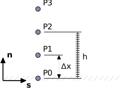
Where the point P2 is taken as reference for stress calculation with the wall model. Pressure is taken from first point at normal direction plus pressure gradient at normal direction, which is estimated from Navier Stokes Equations:

(4)\[ 0 = -\frac{\mathrm{d}p}{\mathrm{d}n}+ \rho \nu \left(\frac{\partial^{2}u_{n} }{\partial n^{2}}\right) \]

The four-point stencil \(2 u_{\mathrm{P0}} - 5 u_{\mathrm{P1}} + 4 u_{\mathrm{P2}} - u_{\mathrm{P3}}\) is the forward second-difference approximating \(\partial^{2}u_{n}/\partial n^{2}\) (the viscous term of the simplified NSE (4)), so it is normalized by \(\Delta x^{2}\). The pressure gradient is then:

(5)\[ \frac{\mathrm{d}p}{\mathrm{d}n} = \rho_{\mathrm{P0}} \nu \left(\frac{2 u_{\mathrm{P0}} - 5 u_{\mathrm{P1}} + 4 u_{\mathrm{P2}} - u_{\mathrm{P3}}}{\Delta x ^{2}}\right) \]

Hence, pressure is calculated as:

(6)\[ p_{\mathrm{P0}}= p_{\mathrm{P1}} - \rho_{\mathrm{P0}} \nu \left(\frac{2 u_{\mathrm{P0}} - 5 u_{\mathrm{P1}} + 4 u_{\mathrm{P2}} - u_{\mathrm{P3}}}{\Delta x ^{2}}\right) \]

Since \(p = \rho c_{s}^{2}\), the pressure at \(\mathrm{P0}\) is estimated as:

(7)\[ \rho_{\mathrm{P0}} = \rho_{\mathrm{P1}}\left[1 + \frac{\nu}{c_{s}^{2}} \left(\frac{2 u_{\mathrm{P0}} - 5 u_{\mathrm{P1}} + 4 u_{\mathrm{P2}} - u_{\mathrm{P3}}}{\Delta x ^{2}}\right)\right]^{-1} \]

The rate-of-strain tensor calculation procedure is described in Wall Model section. From calculated macroscopics, the LBM populations can be reconstructed and wall model BC applied.

Use Case

Wall model BCs are adopted when \(\Delta y^{+}\) of a turbulent flow simulation is higher than 15.

---

[1]

Orestis Malaspinas. Increasing stability and accuracy of the lattice boltzmann scheme: recursivity and regularization. 2015. URL: https://arxiv.org/abs/1505.06900, doi:10.48550/ARXIV.1505.06900.