Surface Coefficients

The end product of a wind-engineering simulation is rarely a velocity field; it is a set of dimensionless coefficients that an engineer can compare against a wind tunnel, a code, or another simulation. Coefficients matter because they remove the arbitrary choice of reference speed and density: the same building tested at two wind speeds, or simulated in lattice units, collapses onto one curve once the load is divided by the dynamic pressure. This is what lets a result obtained in Nassu’s lattice units be read directly against a full-scale measurement. This page defines the surface coefficients the solver reports and then the extreme-value statistics that turn a fluctuating coefficient history into the design quantities used in CWE practice.

Key idea

Dividing a load by the dynamic pressure \(0.5\rho_{0}U_{\mathrm{ref}}^{2}\) removes the arbitrary choice of reference speed and density, so the same body at different speeds, or simulated in lattice units, collapses onto one curve. A result obtained in Nassu’s lattice units then reads directly against a full-scale wind-tunnel measurement, provided the same \(U_{\mathrm{ref}}\) normalizes every coefficient.

The quantities of interest on an immersed boundary are pressure and skin coefficient. On a solid node, they’re defined by

(1)\[\begin{split} \begin{aligned} &C_{p}=\frac{p-p_{0}}{0.5\rho_{0}U_{\mathrm{ref}}^{2}}\\ &C_{f}=\frac{\tau_{w}}{0.5\rho_{0}U_{\mathrm{ref}}^{2}} \end{aligned} \end{split}\]

An accurate representation must also reproduce correct values for the rms pressure coefficient, given by:

(2)\[ C_{p}'=\frac{p_{\mathrm{rms}}}{0.5\rho_{0}U_{\mathrm{ref}}^{2}} \]

where \(p-p_{0}=\left(\rho-\rho_{0}\right)c_{s}^{2}\) and \(U_{\mathrm{ref}}\) is the reference inlet velocity.

The pressure coefficient \(C_{p}\) is local: it gives the load at one point on the surface, which is what governs cladding, glazing and roof-fastening design. Integrating the surface pressure (and skin friction) over the whole body collapses the distribution into the force coefficients, the global loads that govern the structure as a whole [1]:

(3)\[\begin{split} \begin{aligned} &C_{\mathrm{d}}=\frac{F_{x}}{0.5\rho_{0}U_{\mathrm{ref}}^{2}A}\\ &C_{\mathrm{l}}=\frac{F_{z}}{0.5\rho_{0}U_{\mathrm{ref}}^{2}A} \end{aligned} \end{split}\]

where \(F_{x}\) is the force aligned with the incoming wind (drag), \(F_{z}\) is the vertical force (lift), and \(A\) is a reference area.

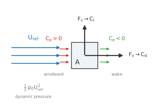
Force and pressure coefficients on a bluff body. The pressure coefficient \(C_{p}\) is a local surface quantity; integrating the pressure and skin friction over the surface gives the global drag \(C_{\mathrm{d}}\) and lift \(C_{\mathrm{l}}\), each normalised by the dynamic pressure \(0.5\rho_{0}U_{\mathrm{ref}}^{2}\) and a reference area \(A\). All coefficients must share the same \(U_{\mathrm{ref}}\) to be comparable.

The same dynamic pressure \(0.5\rho_{0}U_{\mathrm{ref}}^{2}\) normalizes both the local and the global coefficients, which is why a single reference velocity, the mean speed at building height in the CWE convention [1], must be chosen and reported consistently for every coefficient on the page. In a turbulent flow each of these coefficients is itself a fluctuating signal, so the mean \(\bar{C}_{p}\) and the rms \(C_{p}'\) of Eq. (2) are the first two moments of that signal, and the extremes discussed below are its tails.

Note

The skin coefficient of Eq. (1) is multi-directional, that is, it is oriented by a tangential velocity direction. If uni-directional coefficients are to be obtained, the wall shear stress has to be replaced by \(\tau_{xy}\), \(\tau_{xz}\) or \(\tau_{yz}\).

Note

The calculation of skin and pressure coefficients is performed in post-processing for the current solver.

Surface pressure

In the current IBM formulation, there are fluid grid nodes contained inside the Lagrangian mesh. When measuring the pressure, those nodes have to be disregarded since they don’t take effective part in the simulation. The figure below highlights an IBM point with its nearest grid nodes:

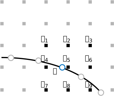
Lima E Silva et al.[2] consider the pressure in a surface point of solid body as the value of nearest grid node external to the mesh. Alternative accurate schemes as in S et al.[3] use geometric interpolation of nearest external nodes using weights inversely proportional to the point distance. From this perspective, the pressure at \(\mathbf{X}\) can be written as:

(4)\[ p\left(\mathbf{X}\right)=\frac{\sum_{n=1}^{N}\left(p\left(\mathbf{x}_{n}\right)/||\mathbf{x}_{n}-\mathbf{X}||\right)}{\sum_{n=1}^{N}\left(1/||\mathbf{x}_{n}-\mathbf{X}||\right)} \]

Extreme and peak coefficients

The mean and rms describe the typical state of the load, but structural failure is driven by the rare events in the tails: the single strongest suction that peels a roof, the largest along-wind gust on a tower. A turbulent coefficient is non-Gaussian at exactly these tails, so the mean and rms alone do not predict the peaks, the distribution’s shape must be characterized directly. Two higher moments quantify that shape [4]. The skewness is the normalized third moment and measures asymmetry: a strongly negative skewness on a leeward or roof region signals that large negative (suction) excursions are more frequent than positive ones, the dangerous case for uplift. The kurtosis is the normalized fourth moment and measures how heavy the tails are: a kurtosis above the Gaussian value of 3 means extreme events occur more often than a normal distribution would predict. In Oliveira et al.[1] the skewness and kurtosis of \(C_{p}\) are reported probe by probe alongside the mean and rms, with the note that kurtosis, being a higher-order statistic dominated by rare events, requires the longest averaging window to converge.

Reporting the largest observed value of a finite record is not robust, because a longer record simply finds a larger maximum. CWE practice therefore estimates a peak that corresponds to a defined reference duration and a defined probability of exceedance, following the Cook-Mayne approach [5]. The procedure used to validate Nassu [1] is representative: the coefficient history is smoothed with a moving average (to a fixed full-scale gust duration), split into several equal sub-intervals, the maximum and minimum of each sub-interval are extracted, those extremes are fitted to a Gumbel distribution, and the fitted mode is rescaled to the target reference duration. A chosen non-exceedance probability on the fitted distribution then defines the design peak coefficient. This gives a peak that is reproducible and statistically meaningful rather than an accident of record length, and it is the quantity that should be compared against wind-tunnel peaks.

Warning

A subtle trap: peaks need the longest window and the finest mesh

Peak coefficients are the slowest statistic to converge and the most sensitive to resolution: under-resolved LES filters out the smallest scales that carry the sharpest pressure spikes, which tends to underestimate the strongest negative (suction) peaks [1]. A peak that still moves as the averaging window or the mesh is refined is a convergence or resolution signal, not necessarily a modeling error.

---

[1] (1,2,3,4,5)

Waine Oliveira, Rodrigo S. Romanus, and Alan Lugarini. Nassu: a high performance LES solver for computational wind engineering. Journal of Wind Engineering and Industrial Aerodynamics, 274:106465, 2026. doi:10.1016/j.jweia.2026.106465.

[2]

A.L.F. Lima E Silva, A. Silveira-Neto, and J.J.R. Damasceno. Numerical simulation of two-dimensional flows over a circular cylinder using the immersed boundary method. Journal of Computational Physics, 189(2):351–370, 2003. URL: https://www.sciencedirect.com/science/article/pii/S0021999103002146, doi:https://doi.org/10.1016/S0021-9991(03)00214-6.

[3]

Anand Bharadwaj S, Santanu Ghosh, and Cibin Joseph. Interpolation techniques for data reconstruction at surface in immersed boundary method. In 55th AIAA Aerospace Sciences Meeting. American Institute of Aeronautics and Astronautics, jan 2017. URL: https://doi.org/10.2514/6.2017-1427, doi:10.2514/6.2017-1427.

[4]

Stephen B. Pope. Turbulent Flows. Cambridge University Press, 2000. doi:10.1017/CBO9780511840531.

[5]

N. J. Cook and J. R. Mayne. A novel working approach to the assessment of wind loads for equivalent static design. Journal of Wind Engineering and Industrial Aerodynamics, 4(2):149–164, 1979. doi:10.1016/0167-6105(79)90043-6.