The thermal modeling hierarchy

A buoyant flow couples temperature back to the fluid through two physically distinct mechanisms, and keeping them apart is the key to reading any thermal LBM:

• a buoyancy body force, which drives the flow because a warm parcel is lighter than its surroundings, and

• a thermodynamic coupling, which ties density, temperature and pressure together through an equation of state, so that heating a parcel makes it expand.

The first mechanism alone is enough when the density barely moves; the second becomes unavoidable once the temperature difference is large enough to change the density by an appreciable fraction. How strongly the density responds to temperature therefore sets which model is appropriate, and that single question orders the thermal capability into three nested regimes. Each adds to the one below it and is valid over a wider band of temperature variation.

Route	Density	Temperature couples through	Valid for
Constant-density Boussinesq	constant \(\rho_0\)	buoyancy body force \(-\rho_0\,\beta\,(T-T_{\text{ref}})\,G_\alpha\)	small \(\Delta T\) (small density variation)
Weakly-compressible thermal	\(\rho = \sum_i f_i\)	\(\theta\) in the equilibrium, giving \(p = \rho c_s^2(1+\theta)\)	moderate density variation, \(\mathrm{Ma} < 0.1\)
Variable-density low-Mach	\(\rho = P/(rT)\) from the EOS	density slaved to temperature; buoyancy \((\rho - \rho_\infty)\,G_\alpha\)	large density ratio (fire-scale)

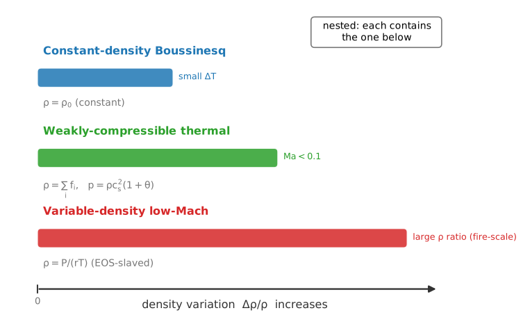
The three thermal regimes ordered by how much the density varies. Each route’s validity band starts at zero density variation and extends further than the one below it, so the regimes are nested: constant-density Boussinesq (small temperature difference), weakly-compressible thermal (moderate variation, bounded by \(\mathrm{Ma} < 0.1\)), and variable-density low-Mach (large density ratio, fire-scale). The route is chosen by the expected density variation, not by the absolute temperature.

The production thermal route is the constant-density Boussinesq one

For the atmospheric, urban and indoor-convection flows Nassu targets, density variation is small and the first route is sufficient and preferred. Temperature is transported as a passive scalar on its own DDF lattice and feeds back through the single buoyancy force, with the fluid collision operator untouched. This is the route documented on the scalar-transport thermal page. The two stronger routes below extend the model toward larger density variation, each with its own validity envelope and its own in-regime benchmark.

Constant-density Boussinesq

In the Boussinesq regime the density is held at a constant reference \(\rho_0\) everywhere it acts as inertia, and its dependence on temperature is retained in one place only: the gravity term, where it produces buoyancy. The temperature obeys a plain advection-diffusion equation and pushes back on the fluid through the body force

(1)\[ F^{\text{buoy}}_\alpha = -\rho_0\, \beta\, (T - T_{\text{ref}})\, G_\alpha, \]

with \(\beta\) the thermal expansion coefficient and \(G_\alpha\) the gravitational acceleration vector. The fluid equilibrium keeps \(\rho_0\); the temperature never enters it. This reduction is derived from the full energy equation on the energy-equation page, and its lattice realization (the DDF scalar plus the Guo buoyancy force) is the scalar-transport thermal route. It is exact in the limit \(\beta\,\Delta T \ll 1\) and models the buoyant driving but neither thermal expansion nor compressibility.

Weakly-compressible thermal

The next regime lets the temperature enter the equilibrium itself. Writing the temperature deviation \(\theta = T/T_0 - 1\) into the equilibrium stress through a \(\rho\,\theta\,\delta_{\alpha\beta}\) term promotes the lattice equation of state from its isothermal form \(p = \rho c_s^2\) to

(2)\[ p = \rho\, c_s^2\,(1 + \theta). \]

The density is still the streamed zeroth moment \(\rho = \sum_i f_i\), and the Mach number must stay below the usual \(\mathrm{Ma} < 0.1\) weakly-compressible threshold. The equilibrium gains the temperature through its rank-2 (\(\rho c_s^2 \theta\,\delta_{\alpha\beta}\)) and rank-3 moments; the full derivation, together with the viscosity correction \(\eta = \rho c_s^2 \Delta t\,(1/\omega - 1/2)(\theta+1)\) and the thermal LES relaxation, is on the compressible LBM page. This is a subset of that page’s machinery: the temperature enters the equilibrium and the pressure, but the energy is supplied by an outer field rather than the entropy equation, and no shock-capturing term is needed in the weakly-compressible regime.

The non-equilibrium does not need a separate temperature term

A natural implementation question is whether the non-equilibrium reconstruction needs its own explicit \(\theta\) contribution to match the equilibrium. It does not. The non-equilibrium is the deviation of the populations from the temperature-dependent equilibrium, \(f_i^{\text{neq}} = f_i - f_i^{\text{eq}}(\theta)\), so the temperature enters it only through the equilibrium it is measured against. The single explicit thermal addition on the standard sets is the third-moment correction \(\Psi\) folded into \(\Pi^{\text{neq}}\) on the compressible LBM page (which on D3Q27 reduces to the lone \(\Psi_{\alpha\alpha\alpha}\) term); there is no separate rank-2 thermal term to add to the non-equilibrium.

Setting \(\theta = 0\) recovers the isothermal development exactly, so the coupling is strictly opt-in (the theta_cte flag): with the isothermal production default every emitted kernel is byte-for-byte unchanged, and the thermal terms appear only when a temperature field is present.

D3Q27 carries the thermal terms without lattice corrections

Thermal LBM formulations built on D3Q19 (as in Taha et al.[1]) carry explicit third- and fourth-order Hermite correction terms to compensate for the incomplete Hermite basis on that lattice. Nassu’s production set is D3Q27, on which the full Hermite basis is exact [2]. The thermal terms drop straight into the complete-basis equilibrium and non-equilibrium without those lattice-specific corrections (the single residual D3Q27 third-moment correction is given on the compressible LBM page), so that part of the D3Q19 derivation is not needed here.

Two points fix how this route relates to the rest of the model:

• The temperature deviation is supplied, not solved inside the fluid. \(\theta\) is an input macroscopic provided by an outer transported field, either the passive scalar acting as a reduced temperature or a dedicated energy field. The fluid LBM consumes \(\theta\) and advects it; it never grows its own temperature solver, and the producing field rides the existing transported-field path.

• The equilibrium coupling and the buoyancy force model distinct terms. The \(\rho\theta\) in the equilibrium is the thermal expansion through the pressure (2); the Boussinesq force (1) is the buoyant driving. They are additive, each representing a different physical effect, and the same physics is not counted twice.

• It is validated in its own regime, not on a fire. Because the equilibrium coupling never activates in a constant-density Boussinesq run (that route keeps \(\rho_0\) in the equilibrium and couples only through the force), this route needs its own in-regime benchmark: a natural-convection / differentially-heated cavity at moderate \(\Delta T\), where the equilibrium pressure coupling is exercised, rather than a fire-scale case that lies outside its envelope.

This route extends Boussinesq to moderate density variation, but it remains a weakly-compressible model: the representable density ratio is bounded by \(\mathrm{Ma} < 0.1\) and by the small-\(\theta\) expansion, so it does not reach the threefold-to-fourfold density change of a fire-scale flow, which is the province of the variable-density route below.

Variable-density low-Mach

The strongest regime makes density a function of temperature through the equation of state, rather than reading it from streaming. This is the closure Taha et al.[1] use for fire-induced flows, and the only one that reaches the large density ratios the two weakly-compressible routes cannot. The rest of this section gives it at the level of detail an implementation needs; the algebra that is specific to Nassu’s lattice is referenced back to the compressible LBM page, and the algebra that is specific to the pressure-based scheme is referenced to the equations of Taha et al.[1] by number.

Governing equations

The target is the low-Mach (acoustically filtered) form of the compressible equations, with density varying but pressure split. Continuity keeps the density derivative,

(3)\[ \partial_t \rho + \partial_\alpha(\rho\, u_\alpha) = 0, \]

momentum carries the hydrodynamic-pressure gradient, the deviatoric stress \(\tau_{\alpha\beta}\) and the buoyancy term,

(4)\[ \partial_t(\rho\, u_\alpha) + \partial_\beta(\rho\, u_\alpha u_\beta) = -\,\partial_\alpha p^h + \partial_\beta \tau_{\alpha\beta} + (\rho - \rho_\infty)\, G_\alpha, \]

and temperature is advanced by the energy equation (the enthalpy form of Taha et al.[1], their Eq. 4), which in the low-Mach limit with \(\mathrm{d}P/\mathrm{d}t = 0\) reduces to conduction-advection with a volumetric source,

(5)\[ \rho\, c_p \left( \partial_t T + u_\alpha \partial_\alpha T \right) = \partial_\alpha\!\left( k\, \partial_\alpha T \right) + S . \]

The set is closed by the ideal-gas equation of state (Taha et al.[1], Eqs. 12 and 32),

(6)\[ P = \rho\, r\, T \qquad\Longleftrightarrow\qquad \rho = \frac{P}{r\,T}, \]

with \(r\) the specific gas constant. Buoyancy is the exact

(7)\[ F^{\text{buoy}}_\alpha = (\rho - \rho_\infty)\, G_\alpha, \]

of which the Boussinesq force (1) is the linearized small-\(\Delta T\) limit, \(\rho - \rho_\infty \approx -\rho_0\,\beta\,(T - T_{\text{ref}})\).

The thermodynamic / hydrodynamic pressure split

The pressure is split into a spatially uniform thermodynamic pressure \(P(t)\), which appears only in the equation of state (6), and a hydrodynamic pressure \(p^h(\mathbf{x},t)\), which drives the flow in (4). Filtering acoustics is exactly the statement that \(P\) does not vary in space. Its evolution in time depends on the boundaries:

• Open domain (the fire-plume and doorway cases): mass leaves and enters freely, so \(P\) is pinned to the ambient and \(\mathrm{d}P/\mathrm{d}t = 0\) (Taha et al.[1], Eq. 3).

• Closed domain: \(P(t)\) is fixed instead by global mass conservation, \(P(t) = m_{\text{tot}}\, r \big/ \int_V T^{-1}\,\mathrm{d}V\), and must be recomputed each step.

The pressure-based LBM variable and the zeroth-moment reinterpretation

The single structural change to the fluid core is what the streamed populations encode. In the pressure-based scheme the LBM solves for the hydrodynamic pressure, carried as the reduced hydrodynamic pressure (Taha et al.[1], Eq. 33)

(8)\[ \theta^{p} \equiv \frac{p^h}{\rho\, c_s^2}, \]

so that the zeroth moment of \(f_i\) returns \(\theta^{p}\) (hydrodynamic pressure), not density (its update is their Eq. 34). Density is then not obtained from streaming; it is closed algebraically from the equation of state (6) using the temperature from the energy field. The velocity is the first moment corrected by the half-step buoyancy force in the usual Guo sense (Taha et al.[1], Eq. 35). This reinterpretation of the zeroth moment is the whole of the departure from Nassu’s mechanical core: streaming, regularization, the multiblock communication and the LES relaxation are untouched, because they act on populations and on \(\rho\), \(u_\alpha\), \(\Pi^{\text{neq}}\) as before, with \(\rho\) now supplied by (6) instead of by the population sum.

Taha’s \(\theta\) is a pressure, not a temperature

In Taha et al.[1] the symbol \(\theta \equiv p^h/(\rho c_s^2)\) denotes the reduced hydrodynamic pressure (8), the lattice pressure variable, whereas in Nassu \(\theta = T/T_0 - 1\) is the temperature deviation. The \(\rho\theta\) that appears in both equilibria is a coincidence of notation, not the same quantity. The transferable content of the reference is the equation of state (6), the pressure split and the moment reconstruction, not a term-for-term copy of their equilibrium: their Eqs. 28-29 carry explicit third- and fourth-order Hermite corrections for D3Q19, which Nassu’s D3Q27 complete basis makes unnecessary (the residual D3Q27 third-moment correction is on the compressible LBM page).

The energy field

Temperature (5) is a transported field, and it rides the existing transported-field path (the same MacrsHandler / capability-flag abstraction the passive scalar uses), never a forked solver. Two realizations are open and the choice is deliberate:

• a finite-difference update beside the LBM, as Taha et al.[1] solve the enthalpy equation, conducting at a real Prandtl number \(k = \rho c_p \nu/\mathrm{Pr}\); or

• a double-distribution LBM scalar, which departs from the reference but reuses the scalar collision and communication unchanged.

The coupling is two-way: the fluid advects \(T\) through (5), and \(T\) sets the density (6) that feeds back into momentum (4) and the buoyancy (7).

One time step

The update sequence per fluid step, following Taha et al.[1] Section 2, is:

1. collide and stream the fluid populations, recovering the reduced hydrodynamic pressure \(\theta^{p}\) (zeroth moment) and the momentum (first moment);

2. advance the temperature field (5) with the current velocity;

3. update the thermodynamic pressure \(P\) (constant for an open domain, from global mass for a closed one);

4. close the density from the equation of state (6);

5. reconstruct the velocity with the half-step buoyancy force (7), and form the force for the next step.

Because the zeroth moment is reinterpreted and the density is closed externally, this regime touches the fluid core more deeply than the equilibrium coupling above, but the change is localized to those two points; everything else is the shared, single-path machinery.

What the Steckler room fire needs

The Steckler room-fire validation case is a compartment fire: a buoyant plume from an internal heat source vents through a doorway into open ambient, with a density contrast across the doorway well outside the Boussinesq small-\(\Delta T\) envelope. The variable-density low-Mach closure represents the true density field across the doorway, and it maps onto a compartment-fire setup as follows:

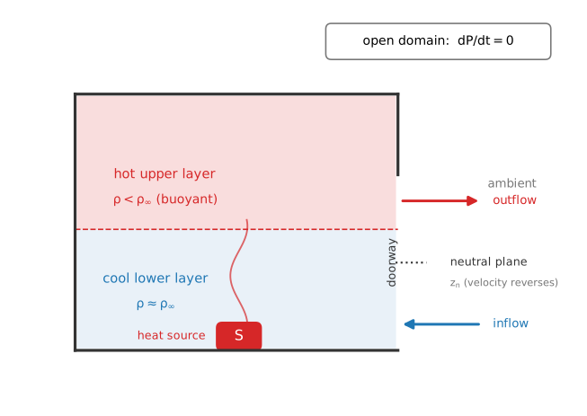
The Steckler compartment-fire doorway exchange, the chapter’s canonical non-Boussinesq worked example. A floor-centred volumetric heat source \(S\) warms a buoyant, density-thinned upper layer (\(\rho < \rho_\infty\)) that spills out the top of the doorway, while ambient air is drawn in through the bottom; the through-door velocity reverses at the neutral plane \(z_n\). The open doorway pins the thermodynamic pressure to ambient, so \(\mathrm{d}P/\mathrm{d}t = 0\).

• The doorway makes the domain open, so \(\mathrm{d}P/\mathrm{d}t = 0\) and the thermodynamic pressure stays at ambient: no global-mass pressure update is needed.

• The fire is the volumetric heat source \(S\) in the energy equation (5), supplied through source_regions; its non-dimensional measure is the heat-release rate \(Q^*_H\) defined on the dimensionless page.

• The balancing recipe is matching \(Q^*_H\) and \(\mathrm{Pr}\), lowering the lattice gravity so the buoyancy velocity stays subsonic, and leaving the Reynolds number reduced, all from the stability page. The variable-density model changes how the density is represented (slaved to temperature rather than frozen), not the strategy for choosing the lattice groups.

• The buoyancy term (7) takes the place of the linearized Boussinesq force, so a doorway density ratio of order two is represented directly instead of through the small-\(\Delta T\) approximation.

The variable-density route therefore needs the variable-density closure plus an energy field for the temperature, with the dimensionless balancing reused unchanged.

Choosing a route

The model is chosen by how much the density is expected to vary, not by the absolute temperature. Small temperature differences (atmospheric stratification, urban heat island, indoor convection) are well served by the constant-density Boussinesq route and should use it. Moderate density variation that still respects \(\mathrm{Ma} < 0.1\) admits the weakly-compressible thermal route. Only the large density ratios of strongly buoyant flows, fire-scale plumes among them, require the variable-density low-Mach closure; a Boussinesq surrogate of such a case captures the qualitative exchange but not the true density field. The differentially-heated cavity validation case is a Boussinesq benchmark by construction and exercises the first route only; a non-Boussinesq cavity at large \(\Delta T\) or a non-reactive density-driven plume (for example a helium plume, where the density contrast comes from molecular weight rather than combustion) sits in the variable-density regime.

---

[1] (1,2,3,4,5,6,7,8,9,10,11)

Mostafa Taha, Song Zhao, Aymeric Lamorlette, Jean-Louis Consalvi, and Pierre Boivin. Large eddy simulation of fire-induced flows using lattice-boltzmann methods. International Journal of Thermal Sciences, 197:108801, 2024. doi:10.1016/j.ijthermalsci.2023.108801.

[2]

Orestis Malaspinas. Increasing stability and accuracy of the lattice boltzmann scheme: recursivity and regularization. 2015. URL: https://arxiv.org/abs/1505.06900, doi:10.48550/ARXIV.1505.06900.