
 AeroSim Docs
Turbulent Channel (Reynolds 2003)
The simulation of a periodic turbulent channel is also used for validation of the equilibrium wall model implemented with the thin boundary layer (TBL) equation. A friction Reynolds number of 2003 is fixed for this case. The reference article used for comparison of results is Han et al., 2020. The pressure gradient is estabilished through a constant body force.
[1]:
from nassu.cfg.model import ConfigScheme

filename = (
    "validation/turbulence/02_turbulent_channel_flow/02.1_turbulent_channel_flow_wm.nassu.yaml"
)

sim_cfgs = ConfigScheme.sim_cfgs_from_file_dct(filename)
[2]:
sim_cfg = next(
    sim_cfg
    for (name, _), sim_cfg in sim_cfgs.items()
    if sim_cfg.name == "periodicTurbulentChannel"
)
sim_cfg_wm = next(
    sim_cfg
    for (name, _), sim_cfg in sim_cfgs.items()
    if sim_cfg.name == "periodicTurbulentChannelMultilevel"
)
sim_cfg_wm_mb = next(
    sim_cfg
    for (name, _), sim_cfg in sim_cfgs.items()
    if sim_cfg.name == "periodicTurbulentChannelNoWM"
)
sim_cfgs_use = {"ref": sim_cfg, "wm": sim_cfg_wm, "mb": sim_cfg_wm_mb}
Functions to use for turbulence channel processing
[3]:
import pathlib

import numpy as np
import pandas as pd

import nassu.viz as common

common.use_style()


def get_experimental_profiles(reynolds_tau: float) -> dict[str, pd.DataFrame]:
    files_tau: dict[float, dict[str, str]] = {
        2003: {
            "ux": "Re_tau_2003_u_avg.csv",
            "ux_rms": "Re_tau_2003_u_rms.csv",
            "uy_rms": "Re_tau_2003_v_rms.csv",
            "uz_rms": "Re_tau_2003_w_rms.csv",
        },
    }

    files_get = files_tau[reynolds_tau]
    vals_exp: dict[str, pd.DataFrame] = {}
    for name, comp_file in files_get.items():
        filename = (
            pathlib.Path("validation/turbulence/02_turbulent_channel_flow/reference") / comp_file
        )
        df = pd.read_csv(filename, delimiter=",")
        vals_exp[name] = df
    return vals_exp


# One cached wall-normal (z) centre-line probe per simulation's statistics
# export, reused for every macroscopic instead of re-probing per call. The
# wall-modelled channel walls are inset by 4 cells, so the line spans z in
# [4, z/2] over z-8 samples (no cell-centre offset, matching the original).
_line_probes: dict[str, common.LineProbe] = {}


def _line_probe(sim_cfg) -> common.LineProbe:
    if sim_cfg.name not in _line_probes:
        ds = sim_cfg.domain.domain_size
        _line_probes[sim_cfg.name] = common.LineProbe.from_export(
            sim_cfg.output.exports["default_stats"].volumes["default_stats"].stats,
            sim_cfg.n_steps + 1,
            (ds.x // 2, ds.y // 2, 4),
            (ds.x // 2, ds.y // 2, ds.z // 2),
            ds.z - 8,
            cell_offset=0.0,
        )
    return _line_probes[sim_cfg.name]


def get_macr_compressed(sim_cfg, macr_name: str, is_2nd_order: bool) -> np.ndarray:
    probe = _line_probe(sim_cfg)
    ds = sim_cfg.domain.domain_size
    norm_pos = (probe.sample_points[:, 2] - 4) / (ds.z - 8)
    name = macr_name if not is_2nd_order else f"{macr_name}_2nd"
    return np.array([norm_pos, probe.sample(name)])
[4]:
y, ux_avg = get_macr_compressed(sim_cfg, "ux", is_2nd_order=False)
Results
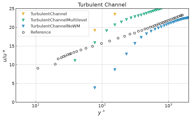
The average velocity profile is shown for the case. It can be seen a good approximation of desired profile when using the wall model.
[5]:
import matplotlib.pyplot as plt

reynolds_tau = 2003
# TODO(#750): verify this normalization before migrating to common.friction_velocity.
# u_ref = 0.00225 is ~9% below the force-implied friction velocity
# u* = sqrt(F * delta) ~ 0.00246 (F = 1.898e-7, half-height delta ~ 28-32 in z
# for the wall-inset channel). This is the residual normalization question
# flagged on #750; re-run on GPU and check against the DNS reference, then
# replace with common.friction_velocity(sim_cfg, geometry="channel", length=...).
u_ref = 0.00246

fig, ax = plt.subplots(1, 1, figsize=(8, 5))

sim_colors = [common.colors.sim, common.colors.green, common.colors.blue]


for i, (sim_cfg, c) in enumerate(zip(sim_cfgs_use.values(), sim_colors)):
    height_scale = common.wall_units_scale(sim_cfg, u_ref)
    name = sim_cfg.name.removeprefix("periodic")

    analytical_values = get_experimental_profiles(reynolds_tau)

    y, ux_avg = get_macr_compressed(sim_cfg, "ux", is_2nd_order=False)
    if not sim_cfg.name.endswith("Multilevel"):
        y, ux_avg = y[::2], ux_avg[::2]

    ux_avg /= u_ref
    y *= height_scale * (sim_cfg.domain.domain_size.z - 8)

    exp_y = analytical_values["ux"]["y+"]
    exp_ux_avg = analytical_values["ux"]["u/u*"]

    ax.plot(
        y,
        ux_avg,
        marker="v",
        fillstyle="none",
        linestyle="none",
        color=c,
        markeredgewidth=1.7,
        label=f"{name}",
    )

ax.plot(exp_y, exp_ux_avg, **common.markers.exp(shape="o"), label="Reference")

ax.set_title("Turbulent Channel")

ax.legend(loc="upper left")
ax.set_xlim(5, 2000)
ax.set_ylim(0, 25)
ax.set_xscale("symlog")
ax.set_ylabel("$u/u*$")
ax.set_xlabel("$y^+$")

plt.tight_layout()
plt.show(fig)
The results of the \({\mathrm{u_{rms}}}\) velocity profiles shown below also indicate a good representation with the multilevel approach.
[6]:
fig, axes = common.fig_triple()

vel_name_map = {"ux": "u", "uy": "v", "uz": "w"}
vel_colors = {"ux": common.colors.sim, "uy": common.colors.blue, "uz": common.colors.green}
vel_exp_markers = {"ux": "o", "uy": "^", "uz": "s"}

for i, sim_cfg in enumerate(sim_cfgs_use.values()):
    name = sim_cfg.name.removeprefix("periodic")
    for macr_name in ("ux", "uy", "uz"):
        macr_compr_rms = get_macr_compressed(sim_cfg, macr_name, is_2nd_order=True)
        macr_compr_avg = get_macr_compressed(sim_cfg, macr_name, is_2nd_order=False)

        y = macr_compr_rms[0].copy()
        vel_2nd = macr_compr_rms[1].copy()
        vel_avg = macr_compr_avg[1].copy()
        vel_rms = (vel_2nd - vel_avg**2) ** 0.5

        vel_rms /= u_ref
        y *= height_scale * (sim_cfg.domain.domain_size.z - 8)
        # Remove wall value
        vel_rms = vel_rms[::2]
        y = y[::2]

        c = vel_colors[macr_name]
        name_vel = vel_name_map[macr_name]
        df = analytical_values[f"{macr_name}_rms"]
        exp_y = df["y+"]
        exp_rms = df[f"{name_vel}'/u*"]

        axes[i].plot(
            y,
            vel_rms,
            marker="v",
            linestyle="none",
            color=c,
            markeredgewidth=1.7,
            label=f"{name} {name_vel.upper()}",
        )
        axes[i].plot(
            exp_y,
            exp_rms,
            marker=vel_exp_markers[macr_name],
            fillstyle="none",
            linestyle="none",
            color=c,
            markeredgewidth=1.7,
            alpha=0.6,
            label=f"Ref. {name_vel.upper()}",
        )

    axes[i].set_title(f"{name}")
    axes[i].legend()
    axes[i].set_xlim(10, 2000)
    axes[i].set_ylim(0, 3.5)
    axes[i].set_xlabel("$y^+$")

plt.tight_layout()
plt.show(fig)
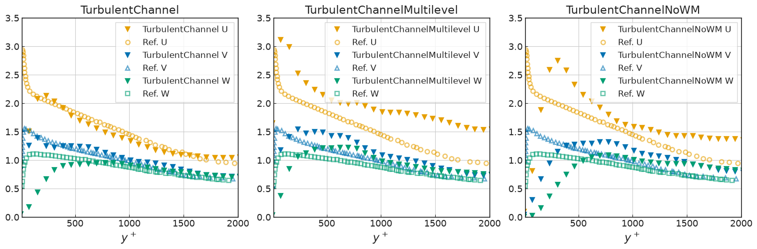
It can be seen good approach of results with the use of wall model and subsequent combination with multigrid approach. As the shell point becomes nearer the surface for a high refinement, the first point velocity becomes a little smaller than for a coarser refinement.
Flow field
Instantaneous velocity magnitude on the wall-modelled channel planes (plane_series): the streamwise / wall-normal mid-plane and the wall-parallel plane above the wall-model matching height.
[7]:
from nassu import viz

viz.enable_offscreen()

PANEL = (840, 320)
cfg = sim_cfgs["periodicTurbulentChannel", 0]
domain = (168.0, 168.0, 64.0)

panels = [
    viz.Panel(
        "mid-channel",
        viz.PlaneSource.from_cfg(cfg, series="plane_series", plane="mid_channel"),
        viz.frame_domain(domain, "y", panel=PANEL, slice_coord=84.0),
    ),
    viz.Panel(
        "near-wall",
        viz.PlaneSource.from_cfg(cfg, series="plane_series", plane="near_wall"),
        viz.frame_domain(domain, "z", panel=PANEL, slice_coord=8.0),
    ),
]
steps = [panels[0].source.steps[-1]]
plotter = viz.render_grid(
    panels,
    steps=steps,
    scalar="u_mag",
    cmap="viridis",
    clim=(0.0, 0.06),
    bar_title="|u|",
    panel_size=PANEL,
)
plotter.show()
2026-07-23 02:38:13.125 (   2.826s) [    7819A4F26B80]vtkXOpenGLRenderWindow.:1460  WARN| bad X server connection. DISPLAY=
/tmp/ipykernel_2102530/83295274.py:31: UserWarning: Using static image for notebook display.
Install trame for interactive backends: pip install "pyvista[jupyter]"
  plotter.show()

Version
[8]:
sim_info = sim_cfg.output.read_info()

nassu_commit = sim_info["commit"]
nassu_version = sim_info["version"]
print("Version:", nassu_version)
print("Commit hash:", nassu_commit)
Version: 2.0.0a7
Commit hash: 5e47f2762575c2d285254d36bfd354b6af09fda1
Configuration
[9]:
from IPython.display import Code

Code(filename=filename)
[9]:
variables:
  # Domain size
  ds:
    x: 168
    y: 168
    z: 64
  # Equation-based ("cold") start - self-contained, no external
  # artefact. The streamwise field is an analytic Reichardt mean
  # profile mirrored across both walls (wall distance in viscous
  # units y+ = (u*/nu) * min(y, NY - y) = 4.5 * min(y, NY - y)),
  # seeded with wall-enveloped multi-mode sinusoidal perturbations
  # (streamwise streaks plus cross-flow rolls carrying wall-normal
  # velocity) at ~10% intensity to break the x/z symmetry and trip
  # transition to turbulence. The sin(pi*y/NY) envelope vanishes at
  # both no-slip walls. The scalar is initialised separately via its
  # `initial_field` ramp.
  init:
    ds:
      ux: !sub "0.005 * (2.5*log(1 + 0.41*4.5*Min(y, ${ds.y} - y)) + 7.8*(1 - exp(-4.5*min(y, ${ds.y} - y)/11) - (4.5*min(y, ${ds.y} - y)/11)*exp(-4.5*min(y, ${ds.y} - y)/3))) + 0.010*sin(pi*y/${ds.y})*cos(2*pi*5*z/${ds.z}) + 0.006*sin(pi*y/${ds.y})*sin(2*pi*3*x/${ds.x})*cos(2*pi*4*z/${ds.z})"
      uy: !sub "0.006*sin(pi*y/${ds.y})*sin(2*pi*3*x/${ds.x})*cos(2*pi*4*z/${ds.z}) + 0.004*sin(pi*y/${ds.y})*sin(2*pi*2*x/${ds.x})*sin(2*pi*3*z/${ds.z})"
      uz: !sub "0.006*sin(pi*y/${ds.y})*sin(2*pi*3*x/${ds.x})*sin(2*pi*4*z/${ds.z}) - 0.004*sin(pi*y/${ds.y})*cos(2*pi*2*x/${ds.x})*cos(2*pi*3*z/${ds.z})"

simulations:
  - name: periodicTurbulentChannel
    save_path: ./validation/turbulence/02_turbulent_channel_flow/results/periodic
    run_simul: true

    n_steps: 200000
    report:
      frequency: 1000

    domain:
      domain_size:
        x: !math ${ds.x}
        y: !math ${ds.y}
        z: !math ${ds.z}
      block_size: 8
      bodies:
        plane_floor:
          IBM:
            run: true
            cfg_use: plane_cfg
            order: 0
          geometry_path: fixture/stl/abl/ground.stl
          transformation:
            scale: [2, 2, 2]
            translation: [0, 0, 4]
        plane_ceil:
          IBM:
            run: true
            cfg_use: plane_cfg
            order: 0
          geometry_path: fixture/stl/abl/ground.stl
          transformation:
            scale: [2, 2, 2]
            fixed_point: [0, 80, 0]
            rotation: !math [radians(180), 0, 0]
            translation: [0, 0, 60]

    data:
      export_IBM_nodes:
        ibm_exp:
          body_name: plane_floor
          frequency: 5000
      exports:
        default:
          macrs: [rho, u, omega_LES, f_IBM]
          interval:
            frequency: 50000
            lvl: 0
          target:
            volumes:
              default: {}
          outputs:
            instantaneous: true
        default_stats:
          macrs:
            - rho
            - u
          interval:
            frequency: 100
            start_step: 100000
            lvl: 0
          target:
            volumes:
              default_stats: {}
          outputs:
            instantaneous: false
            stats:
              macrs_1st_order:
                - rho
                - u
              macrs_2nd_order:
                - u
        plane_series:
          macrs: [rho, u]
          interval: {frequency: 25000, lvl: 0}
          target:
            planes:
              # Streamwise / wall-normal mid-plane (IBM walls are z-normal).
              mid_channel:
                axis: y
                axis_pos: 84
                dist: 1
              # Wall-parallel plane above the wall-model matching height.
              near_wall:
                axis: z
                axis_pos: 8
                dist: 1
          outputs:
            instantaneous: true

    models:
      precision:
        default: single

      LBM:
        tau: 0.500096682620786
        F:
          x: 1.89820067659664E-07
          y: 0
          z: 0
        vel_set: D3Q27
        coll_oper: RRBGK
      initialization:
        equations:
          rho: "1"
          ux: !sub ${init.ds.ux}
          uy: !sub ${init.ds.uy}
          uz: !sub ${init.ds.uz}

      engine:
        name: CUDA

      LES:
        model: Smagorinsky
        sgs_cte: 0.17

      BC:
        periodic_dims: [true, true, true]

      IBM:
        dirac_delta: 3_points
        forces_accomodate_time: 0
        reset_forces: true
        body_cfgs:
          default:
            n_iterations: 1
            forces_factor: 1.0
          plane_cfg:
            n_iterations: 1
            forces_factor: 0.25
            wall_model:
              name: EqTBL
              dist_ref: 2.0
              dist_shell: 0.25
              start_step: 0
              params:
                z0: 0.00155
                TDMA_max_error: 1e-04
                TDMA_max_iters: 10
                TDMA_min_div: 51
                TDMA_max_div: 51

      multiblock:
        overlap_F2C: 2

  - name: periodicTurbulentChannelMultilevel
    parent: periodicTurbulentChannel
    run_simul: true

    domain:
      refinement:
        static:
          default:
            volumes_refine:
              - start: [0, 0, 0]
                end: [168, 168, 16]
                lvl: 1
                is_abs: true
              - start: [0, 0, 48]
                end: [168, 168, 64]
                lvl: 1
                is_abs: true

  - name: periodicTurbulentChannelNoWM
    parent: periodicTurbulentChannel
    run_simul: true

    models:
      IBM:
        body_cfgs:
          plane_cfg:
            wall_model: