AeroSim Docs
Turbulent Channel Flow
Why this case matters
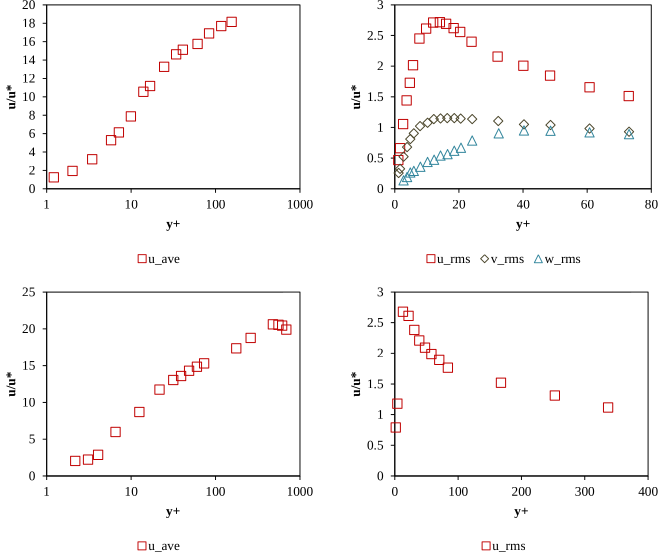
Turbulent channel flow is the most studied wall-bounded turbulent flow and the primary test of whether the LES subgrid model and near-wall treatment produce correct turbulence statistics, not just a correct mean. Because the flow reaches a statistically stationary state that depends only on the friction Reynolds number (2), the simulated mean profile and the velocity fluctuation intensities can be compared directly against reference data. The benchmarks used here, the low-Reynolds DNS of Kim et al.[1] and the experiment of Eckelmann[2] at \(\mathrm{Re}_{\tau} = 142\), provide both first- and second-order statistics across the whole channel half-height. For computational wind engineering this case underpins confidence that a wall-bounded shear layer is resolved or modelled correctly before any building is introduced into the domain.
A turbulent channel flow consists of a transient pressure-driven flow between parallel plates that occurs at high Reynolds number, as illustrated below
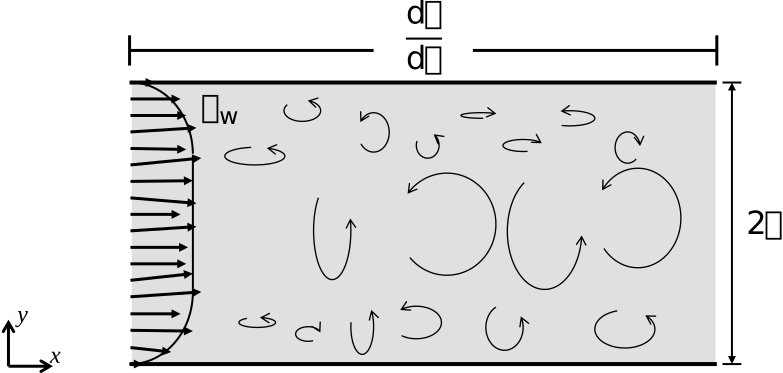
where \(u_{\mathrm{w}}\) is the friction velocity, which is representative of the mean wall shear stress \(\sigma_{\mathrm{w}}\), and is calculated with:
This kind of flow presents eddies that dissipate the energy. The vorticity generation is measured through the flow enstrophy. In spite of this kind of flow being inherently transient, it does present a statistically developed state, to which average and standard deviation velocities are solely dependent on the flow Reynolds number.
The characterization of the flow is usually performed from its friction Reynolds number, given by:
For a turbulent channel flow, the length scale for calculation of the eddy turnover time is \(l=\delta\).
A well established numerical validation of this kind of flow was performed by Kim et al.[1] for a \(\mathrm{Re}_{\tau} = 180\). This work compares its DNS results with the experiment from Eckelmann[2] (\(\mathrm{Re}_{\tau} = 142\)) and supplies useful data for the validation of a turbulent numerical model. Further results for a \(\mathrm{Re}_{\tau} = 520\) are found in Germaine et al.[3], which performs a numerical model validation using experimental data from Lepore and Mydlarski[4].
For an accurate DNS, a grid resolution that accounts for effects of small scale eddies is required. Eggels et al.[5]; Lammers et al.[6] suggest that three grid nodes inside the viscous sublayer (\(y^{+} \leq 8\)) give a sufficient spatial resolution, hence an accurate DNS design requires \(\Delta y^{+} \leq 2.3\), where:
The plots from Eckelmann[2] and Germaine et al.[3] respectively are shown below to illustrated the expected statistics profiles: