Moving Wall¶

Moving wall boundary conditions are those in which a sliding wall is represented, its implementation is usually similar to solid wall implementations, but with a non-null fixed velocity.

Velocity Bounce-Back¶

The velocity bounce-back boundary condition imposes a velocity profile with no transversal components.

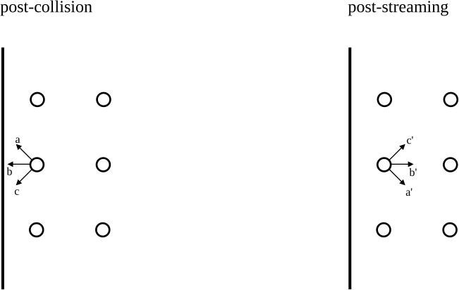
The unknown populations are obtained by reflecting back post-collision populations that entered the wall, just like the HWBB, and then correcting them by

(1)¶\[ f_\bar{i}(t + \Delta t) = f_i^* + \frac{2 w_i \rho_\mathrm{b}\, c_{i\alpha}\, u_{\mathrm{w},\alpha}}{c_s^2} \]

where \(\bar{i}\) is the opposite \(i\)-direction and \(u_{\mathrm{w},\alpha}\) is the prescribed wall velocity, projected onto the lattice direction through \(c_{i\alpha} u_{\mathrm{w},\alpha}\) summed over all components \(\alpha\) (the generic wall-velocity projection, Krüger et al.[1] Eq. 5.26). The correction is added to the opposite (reflected) population \(f_{\bar{i}}\). Notice that the density at the boundary (\(\rho_\mathrm{b}\)) has to be calculated someway. Nassu extrapolates it from the first two fluid nodes along the inward wall normal as \(\rho_\mathrm{b} = \frac{1}{2}\left(3\rho_{b+1} - \rho_{b+2}\right) = \rho_{b+1} + \frac{1}{2}\left(\rho_{b+1} - \rho_{b+2}\right)\), where \(\rho_{b+1}\) and \(\rho_{b+2}\) are the densities at the first and second fluid nodes along the inward wall normal.

Use case

Velocity bounce-back forces a tangential velocity at a wall without restricting the pressure, so it serves both a sliding (moving) wall and a velocity inlet.

Important

Velocity bounce-back steadily adds density to the domain, which can drift the average density and eventually trigger instabilities. This makes it a poor choice at an inlet, where the bias accumulates over the whole run. Where a constant-density inlet is acceptable, use the Uniform velocity BC instead.