Wall Model - LBM boundary condition

The wall function computes a wall stress, but that stress still has to be handed to the flow solver. Nassu offers two coupling routes, and they differ only in where the solid surface lives, not in the modeling described in wall model.

• LBM boundary-condition route (this page). The solid surface is aligned with the lattice and represented by a boundary condition on the wall nodes. This is the natural and most accurate choice when the geometry is flat and grid-aligned, such as the ground plane of an ABL simulation or a wind-tunnel floor. The modeled wall stress enters through the rate-of-strain tensor reconstructed at the wall node, as derived below.

• IBM route (next page). The solid surface is an arbitrary STL body immersed in the lattice and represented by Lagrangian points. This is the choice for the curved and inclined surfaces of real buildings and vehicles, which do not align with a Cartesian grid. There the modeled stress enters as a velocity correction spread back to the fluid through the immersed-boundary interpolation.

Use the boundary-condition route for grid-aligned walls and the IBM route for immersed bodies; the wall function feeding both is identical.

The correction of wall values for a LBM boundary is straightforward, wall density is estimated to be the same as in the first node and the velocity is set to zero.

The reference point \(\mathrm{P_{\mathrm{N}}}\) is assumed to be the second node normal to wall \(\mathrm{P_{2}}\).

A subtle trap: sample the reference point in the log layer

The matching point \(\mathrm{P_{N}}\) must lie where the assumed profile is valid. If the grid is fine enough that \(\mathrm{P_{2}}\) falls inside the viscous or buffer layer, the wall function is being read at a height where its profile shape does not hold, and the recovered friction velocity is biased. This log-layer mismatch is a property of the sampling height, not of the model, and no amount of time-averaging removes it.

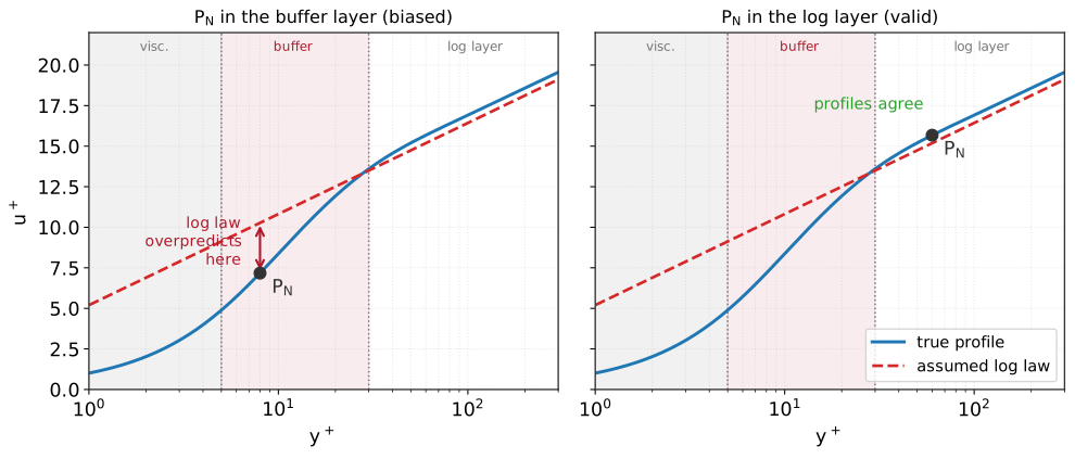
Sampling trap. If the reference point \(\mathrm{P_N}\) falls in the viscous or buffer region (left), the assumed log profile does not hold and the friction velocity is biased; \(\mathrm{P_N}\) must sit in the log layer, \(y^+\) above ~30 (right), where the model is valid.

Using the velocity from \(\mathrm{P_{2}}\), the wall model region is modeled as described in wall model. With the chosen wall model, the velocity at \(\mathrm{P_{1}}\) can be also calculated, and the shear rate at the wall is estimated through a finite difference scheme:

(1)\[ S_{ns}=\frac{\left(-3u_{s}^{(P_{0})}+4 u_{s}^{(P_{1})}-u_{s}^{(P_{2})}\right)}{2\Delta x} \]

The rate-of-strain tensor at \(\mathrm{P_{0}}\) is then built with \(n, s, t\) coordinates. The unit vectors are the surface normal \(\mathbf{n}\), the \(\mathrm{P_{2}}\) tangential velocity direction \(\mathbf{s}\):

(2)\[ \mathbf{s}=\frac{\mathbf{u}_{\mathrm{p_{2}}}-\left(\mathbf{n}\cdot\mathbf{u}_{\mathrm{p_{2}}}\right)\mathbf{n}} {||\mathbf{u}_{\mathrm{p_{2}}}-\left(\mathbf{n}\cdot\mathbf{u}_{\mathrm{p_{2}}}\right)\mathbf{n}||}, \]

and to complete an orthogonal basis, \(\mathbf{t}=\mathbf{s}\times\mathbf{n}/||\mathbf{s}\times\mathbf{n}||\) is perpendicular to \(\mathbf{n}\) and \(\mathbf{s}\).

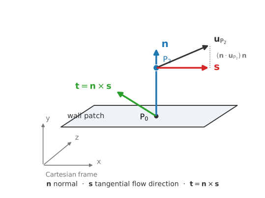
The wall-normal frame used to reconstruct the rate-of-strain. \(\mathbf{n}\) is the surface normal, \(\mathbf{s}\) points along the tangential part of the reference-point velocity, and \(\mathbf{t}=\mathbf{n}\times\mathbf{s}\) completes a right-handed basis; the stress is built in this frame and rotated back to Cartesian.

The rate-of-strain tensor in this coordinate system is written as:

\[ S_{\alpha'\beta'}= \begin{bmatrix} S_{ss} & S_{ns} & S_{ts} \\ S_{sn} & S_{nn} & S_{tn} \\ S_{st} & S_{nt} & S_{tt} \end{bmatrix}= \begin{bmatrix} 0 & S_{ns} & 0 \\ S_{ns} & 0 & 0 \\ 0 & 0 & 0 \end{bmatrix} \]

The wall-normal normal-strain \(S_{nn}\) is set to zero: the wall model reconstructs only the shear component \(S_{ns}\) from the modeled profile, which is the standard equilibrium-wall-model assumption.

The tensor is then adjusted to xyz coordinate system with:

\[ \begin{bmatrix} S_{xx} & S_{xy} & S_{xz} \\ S_{yx} & S_{yy} & S_{yz} \\ S_{zx} & S_{zy} & S_{zz} \end{bmatrix} = \begin{bmatrix} \mathbf{i}\cdot\mathbf{s} & \mathbf{i}\cdot\mathbf{n} & \mathbf{i}\cdot\mathbf{t} \\ \mathbf{j}\cdot\mathbf{s} & \mathbf{j}\cdot\mathbf{n} & \mathbf{j}\cdot\mathbf{t} \\ \mathbf{k}\cdot\mathbf{s} & \mathbf{k}\cdot\mathbf{n} & \mathbf{k}\cdot\mathbf{t} \end{bmatrix} \begin{bmatrix} 0 & S_{ns} & 0 \\ S_{ns} & 0 & 0 \\ 0 & 0 & 0 \end{bmatrix} \begin{bmatrix} \mathbf{i}\cdot\mathbf{s} & \mathbf{i}\cdot\mathbf{n} & \mathbf{i}\cdot\mathbf{t} \\ \mathbf{j}\cdot\mathbf{s} & \mathbf{j}\cdot\mathbf{n} & \mathbf{j}\cdot\mathbf{t} \\ \mathbf{k}\cdot\mathbf{s} & \mathbf{k}\cdot\mathbf{n} & \mathbf{k}\cdot\mathbf{t} \end{bmatrix}^{\mathrm{T}} \]

After adjustment of rate-of-strain, all necessary wall macroscopics are defined and flow evolution can be normally performed. The wall-stress estimate uses the target velocity at \(P_{1}\), so it brings the velocity at the first node close to the desired value.