Atmospheric Boundary Layer

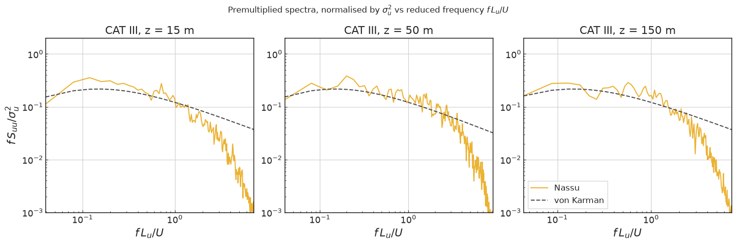
Validation of the neutral atmospheric boundary layer (ABL) over the five terrain categories of EN 1991-1-4 (Eurocode 1), CAT 0 to CAT IV. The case reproduces the published AeroSim ABL validation study and follows the guided-case setup methodology:

• Published validation: https://docs.aerosim.io/validation/cases/vel_turb/abl.html

• Setup guideline: https://docs.aerosim.io/aerosim/guided-cases/ABL/setup.html

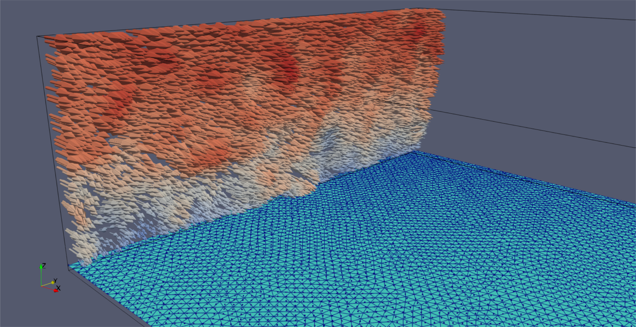
A wind-tunnel-like arrangement is used: the Synthetic Eddy Method (SEM) imposes the target Eurocode logarithmic profile and turbulence at the inlet, and roughness fins on the floor maintain the profile along the fetch:

Inlet turbulence (SEM). The inflow is generated with the synthetic eddy method (SEM): each inlet node is given the target mean velocity profile and Reynolds stress tensor, built from the Eurocode 1 targets and the documented v/w heuristics (Iv = 0.75 Iu, Iw = 0.50 Iu, Lv = 0.25 Lu, Lw = 0.10 Lu; see eurocode.py).

This notebook must be re-executed on a validation-class GPU after the run; the analysis below is inlet-method agnostic (it reads the reference-station time series) and additionally reports the lateral and vertical turbulence intensities against the heuristic targets.

Setup

The floor is an IBM plane at 5.01 lattice units. One level-0 node corresponds to 8 m full-scale (scale 1/8) and the refined slab around the measurement axis runs at level 1, i.e. 4 m - a single resolution. The roughness fins are 6 m wide on a 16 m x 32 m grid; only the fin height changes per category (CAT I: 1 m, CAT II: 2 m, CAT III: 6 m, CAT IV: 10 m; CAT 0 has no fins). The ground plane applies an equilibrium log-law wall model with the category roughness length z0. The outlet is a Neumann condition and the lateral and top faces are free-slip.

Reference conditions: H = 150 m (18.75 lattice units), U_H = 0.06 (lattice), giving Re_H = U_H H / nu = 337,500. Statistics are collected over T / CTS = 128 convective time scales (CTS = H / U_H = 312.5 steps, so 40,000 steps) after a 32 CTS development time.

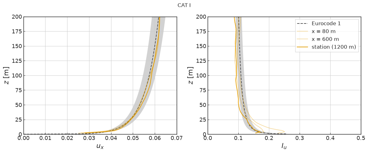
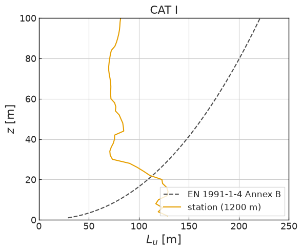
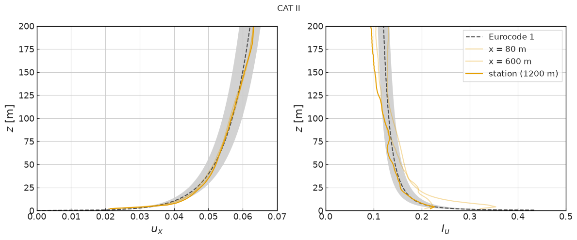
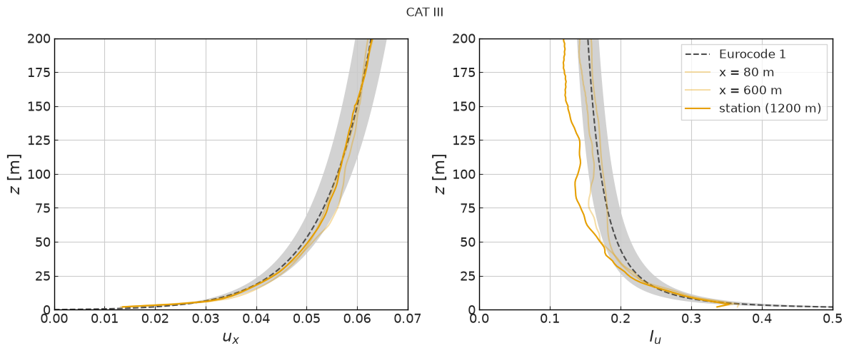
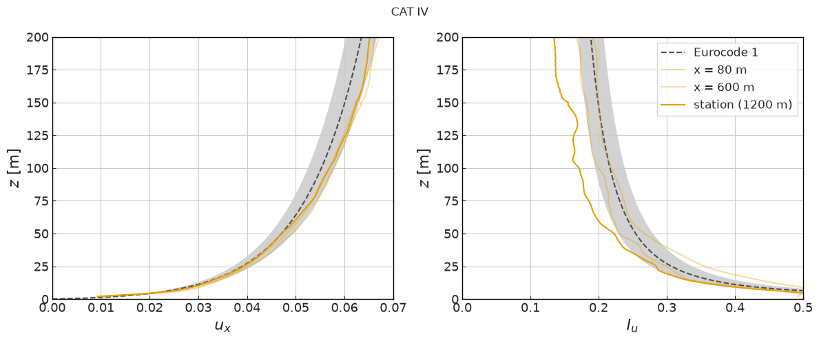
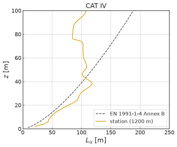
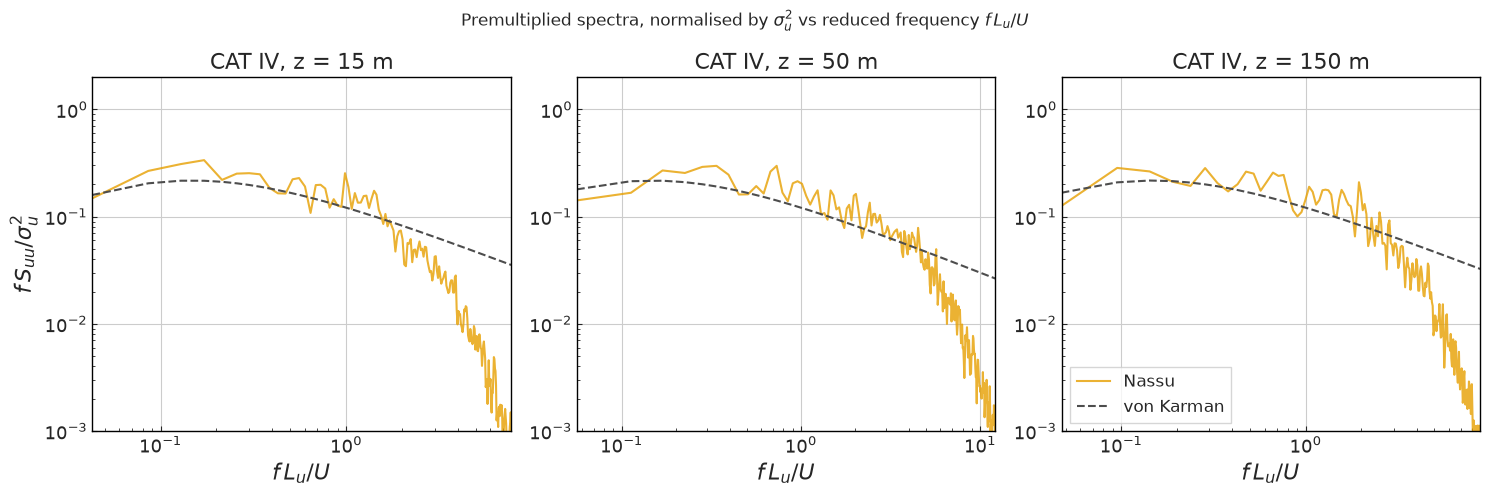
All quantities are reported at the reference station, 1200 m downstream of the inlet, sampled along a vertical line every 2 level-0 steps. Profiles stop at 200 m full-scale - the validity limit of the Eurocode 1 targets:

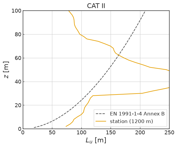
Quantity	Eurocode 1 target	Acceptance
Mean velocity U(z)	logarithmic profile	+-5 %
Turbulence intensity Iu(z)	1 / ln(z / z0)	+-10 %
Integral length scale Lu(z)	EN 1991-1-4 Annex B	qualitative
Energy spectra	von Karman	qualitative

from nassu.cfg.model import ConfigScheme

filename = (
    "validation/wind_engineering/01_atmospheric_boundary_layer/01_atmospheric_flow_sem.nassu.yaml"
)

sim_cfgs = ConfigScheme.sim_cfgs_from_file_dct(filename)

import pathlib

import matplotlib.pyplot as plt
import numpy as np
import pandas as pd

import nassu.viz as common
from nassu.cfg.schemes.simul import SimulationConfigs

common.use_style()

BASE_HEIGHT = 5.01  # IBM ground plane height (lattice units)
M_PER_NODE = 8.0  # full-scale metres per level-0 node (scale 1/8)
H_REF_M = 150.0  # reference height (m)
U_H = 0.06  # lattice velocity at the reference height
DEV_TIME = 10_000  # development steps discarded from every series
SAMPLE_DT = 2.0  # station series sampling interval (level-0 steps)
DEV_SAMPLE_DT = 50.0  # development series sampling interval (level-0 steps)

# sim name -> (label, z0 [m], Eurocode profile CSV)
CATEGORIES = {
    "category_0_s4m": ("CAT 0", 0.003, "profile_log_cat0_H150_Uh0.06"),
    "category_1_s4m": ("CAT I", 0.01, "profile_log_cat1_H150_Uh0.06"),
    "category_2_s4m": ("CAT II", 0.05, "profile_log_cat2_H150_Uh0.06"),
    "category_3_s4m": ("CAT III", 0.3, "profile_log_cat3_H150_Uh0.06"),
    "category_4_s4m": ("CAT IV", 1.0, "profile_log_cat4_H150_Uh0.06"),
}

Processing

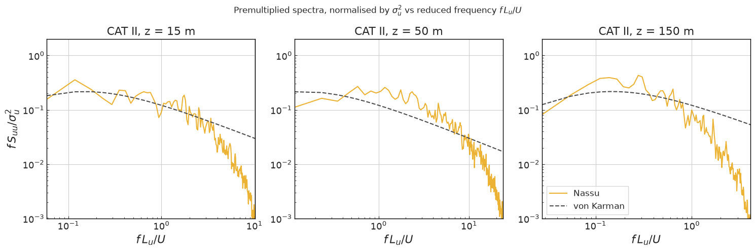
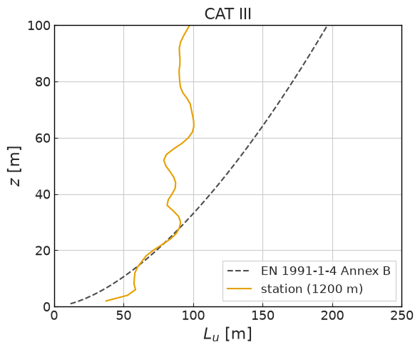
The reference-station line records the ux time series at every height. From a single read all four reported quantities follow: the time mean gives U(z), the standard deviation gives Iu(z), the autocorrelation integrated to its first zero crossing gives the integral time scale (converted to Lu(z) with Taylor’s frozen-turbulence hypothesis), and Welch’s method gives the energy spectra. The statistics helpers live in validation/notebooks/common.py.

_series_cache: dict = {}


def read_line_series(sim_cfg: SimulationConfigs, series: str, line_name: str):
    """Time series of ux at every point of a probe line (statistics window only)."""
    key = (sim_cfg.name, sim_cfg.sim_id, series, line_name)
    if key not in _series_cache:
        # Keep at most one simulation's series in memory.
        if any(k[:2] != key[:2] for k in _series_cache):
            _series_cache.clear()
        line = sim_cfg.output.exports[series].series.lines[line_name]
        df = line.read_full_data("ux")
        df = df[df["time_step"] >= DEV_TIME].sort_values("time_step")
        points = pd.read_csv(line.points_filename)
        _series_cache[key] = (df, points)
    return _series_cache[key]


def line_statistics(
    sim_cfg: SimulationConfigs,
    series: str = "station",
    line_name: str = "reference_station",
    sample_dt: float = SAMPLE_DT,
):
    """Per-height statistics of a vertical probe line: U, Iu and Lu vs height (m)."""
    df, points = read_line_series(sim_cfg, series, line_name)
    stats = []
    for idx, z in zip(points["idx"], points["z"]):
        u = df[str(idx)].to_numpy(dtype=float)
        u_mean = float(u.mean())
        z_m = (z - BASE_HEIGHT) * M_PER_NODE
        if z_m <= 0.0 or u_mean <= 0.0:
            continue
        stats.append(
            {
                "z_m": z_m,
                "u_mean": u_mean,
                "intensity": float(u.std()) / u_mean,
                "length_scale_m": common.integral_length_scale(u, sample_dt) * M_PER_NODE,
            }
        )
    return pd.DataFrame(stats).sort_values("z_m")


def station_spectrum(
    sim_cfg: SimulationConfigs, z_target_m: float, line_name: str = "reference_station"
):
    """Premultiplied, variance-normalised spectrum at the station point closest
    to ``z_target_m``, returned against the reduced frequency ``n L_u / U``.

    The reduced frequency uses the integral length scale ``L_u`` (not the height
    ``z``): that is the length scale the von Karman / EN 1991-1-4 spectrum is
    written in. By Taylor's frozen-turbulence hypothesis ``L_u / U = T_u`` (the
    integral time scale), so ``n L_u / U`` reduces to ``f * T_u``.
    """
    df, points = read_line_series(sim_cfg, "station", line_name)
    z_m = (points["z"] - BASE_HEIGHT) * M_PER_NODE
    row = points.iloc[int((z_m - z_target_m).abs().argmin())]
    u = df[str(int(row["idx"]))].to_numpy(dtype=float)
    f, spec = common.energy_spectrum(u, SAMPLE_DT)
    t_u = common.integral_time_scale(u, SAMPLE_DT)
    f_L = f * t_u  # reduced frequency n L_u / U (Taylor: L_u / U = T_u)
    return f_L, spec * f / u.var()  # premultiplied, variance-normalized: f S / sigma^2


def von_karman_spectrum(fn: np.ndarray) -> np.ndarray:
    """von Karman / EN 1991-1-4 streamwise spectrum in reduced frequency
    ``f_L = n L_u / U``: ``6.8 f_L / (1 + 10.2 f_L)^(5/3)`` (EN 1991-1-4 Eq. B.2)."""
    return 6.8 * fn / (1.0 + 10.2 * fn) ** (5.0 / 3.0)

The Eurocode 1 target curves are the same profiles used to drive the SEM inlet, generated from the EN 1991-1-4 logarithmic equation per category (fixture/SEM/category_vprofile).

comparison_folder = pathlib.Path("fixture/SEM/category_vprofile")

df_eu = {}
for sim_name, (_, z0, csv_name) in CATEGORIES.items():
    df = pd.read_csv(comparison_folder / f"{csv_name}.csv")
    df["Ix"] = (df["Rxx"] / (df["ux"] ** 2)) ** 0.5
    df_eu[sim_name] = df

def plot_profiles(sim_name: str):
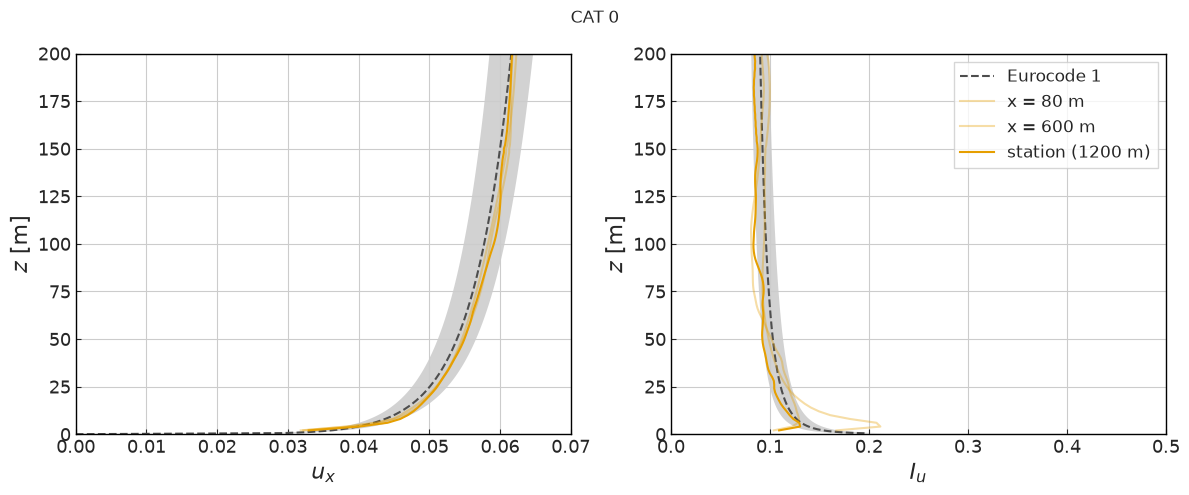
    """U(z) and Iu(z) at the reference station vs the Eurocode 1 targets.

    The shaded bands are the +-5 % (velocity) and +-10 % (intensity) acceptance
    ranges of the published study. Profiles upstream of the station (x = 80 m
    and x = 600 m) show the boundary-layer development along the fetch.
    """
    label, z0, _ = CATEGORIES[sim_name]
    sim_cfg = sim_cfgs[sim_name, 0]
    target = df_eu[sim_name]
    z_t = target["z"].to_numpy()

    fig, ax = common.fig_double()

    ax[0].fill_betweenx(
        z_t,
        0.95 * target["ux"],
        1.05 * target["ux"],
        color=common.colors.exp,
        alpha=0.25,
        linewidth=0,
    )
    ax[0].plot(target["ux"], z_t, **common.markers.exp_line(linestyle="--"), label="Eurocode 1")
    ax[1].fill_betweenx(
        z_t,
        0.9 * target["Ix"],
        1.1 * target["Ix"],
        color=common.colors.exp,
        alpha=0.25,
        linewidth=0,
    )
    ax[1].plot(target["Ix"], z_t, **common.markers.exp_line(linestyle="--"), label="Eurocode 1")

    for series, line_name, line_label, alpha, dt in [
        ("development", "velocity_profile_010", "x = 80 m", 0.35, DEV_SAMPLE_DT),
        ("development", "velocity_profile_075", "x = 600 m", 0.35, DEV_SAMPLE_DT),
        ("station", "reference_station", "station (1200 m)", 1.0, SAMPLE_DT),
    ]:
        profile = line_statistics(sim_cfg, series, line_name, sample_dt=dt)
        kw = common.markers.sim_line(alpha=alpha)
        ax[0].plot(profile["u_mean"], profile["z_m"], **kw, label=line_label)
        ax[1].plot(profile["intensity"], profile["z_m"], **kw, label=line_label)

    ax[0].set_xlabel(r"$u_x$")
    ax[0].set_xlim(0, 0.07)
    ax[1].set_xlabel(r"$I_{u}$")
    ax[1].set_xlim(0, 0.5)
    ax[1].legend()
    for a in ax:
        a.set_ylabel(r"$z$ [m]")
        a.set_ylim(0, 200)
    fig.suptitle(label)
    plt.tight_layout()
    plt.show(fig)


def plot_length_scale(sim_name: str):
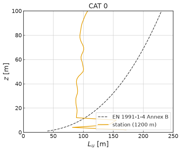
    """Integral length scale Lu(z) at the station vs EN 1991-1-4 Annex B."""
    label, z0, _ = CATEGORIES[sim_name]
    station = line_statistics(sim_cfgs[sim_name, 0])

    fig, ax = common.fig_single()
    z = np.linspace(1.0, 100.0, 200)
    ax.plot(
        common.eurocode_length_scale(z, z0),
        z,
        **common.markers.exp_line(linestyle="--"),
        label="EN 1991-1-4 Annex B",
    )
    ax.plot(
        station["length_scale_m"],
        station["z_m"],
        **common.markers.sim_line(),
        label="station (1200 m)",
    )
    ax.set_ylabel(r"$z$ [m]")
    ax.set_xlabel(r"$L_{u}$ [m]")
    ax.set_ylim(0, 100)
    ax.set_xlim(0, 250)
    ax.legend()
    ax.set_title(label)
    plt.tight_layout()
    plt.show(fig)


def plot_spectra(sim_name: str, heights_m=(15.0, 50.0, 150.0)):
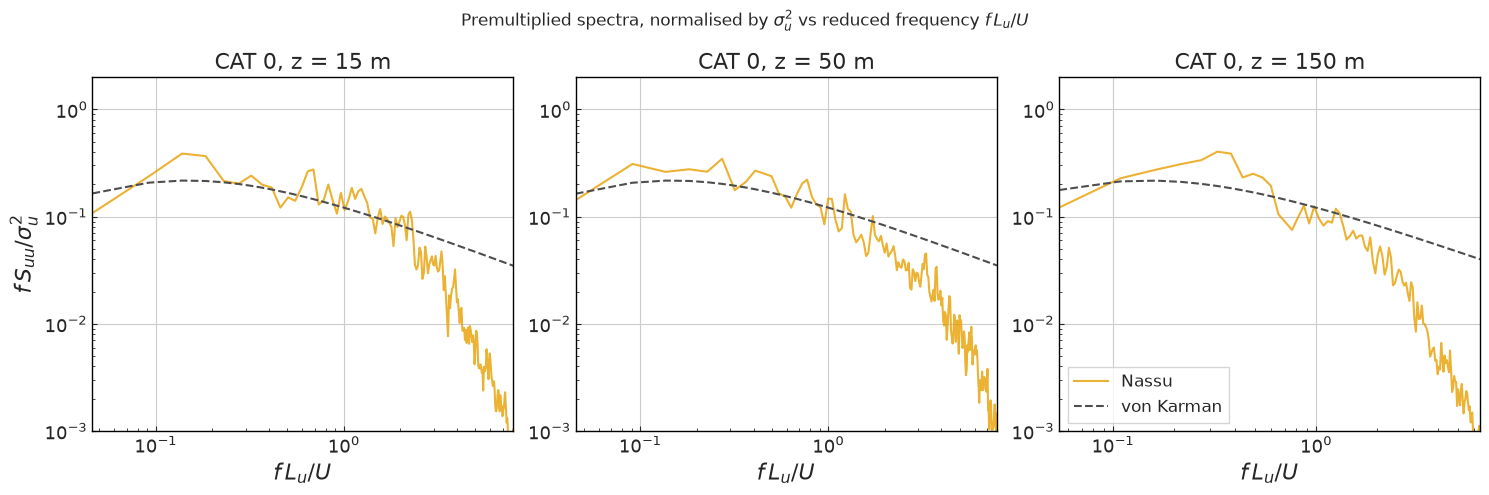
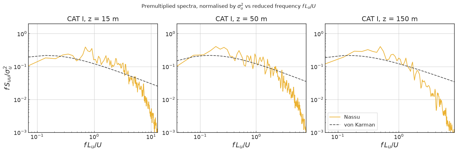
    """Premultiplied, variance-normalised streamwise spectra at the station.

    Both axes are in similarity form so the curve is directly comparable to the
    von Karman model at any height: the frequency is normalised as ``f z / U``
    (Monin coordinate) and the energy as the premultiplied, variance-normalised
    spectrum ``f S_uu / sigma_u^2`` (unit area under d ln f). Axes are clipped to
    the resolved, energy-containing band - the far tail sits below the LES grid
    cutoff and carries no meaningful signal.
    """
    label, _, _ = CATEGORIES[sim_name]
    sim_cfg = sim_cfgs[sim_name, 0]

    fig, ax = common.fig_triple()
    floor = 1e-3
    for i, z_m in enumerate(heights_m):
        fn, spec_n = station_spectrum(sim_cfg, z_m)
        ax[i].plot(fn, spec_n, alpha=0.8, label="Nassu")
        ax[i].plot(
            fn,
            von_karman_spectrum(fn),
            color=common.colors.exp,
            linestyle="--",
            label="von Karman",
        )
        # Clip to the meaningful band: keep only where the resolved spectrum is
        # above the sub-cutoff noise floor.
        keep = (fn > 0) & (spec_n > floor)
        if keep.any():
            ax[i].set_xlim(float(fn[keep].min()), float(fn[keep].max()))
        ax[i].set_ylim(floor, 2.0)
        ax[i].set_title(f"{label}, z = {z_m:.0f} m")
        ax[i].set_xscale("log")
        ax[i].set_yscale("log")
        ax[i].set_xlabel(r"$f\,L_u / U$")
    ax[0].set_ylabel(r"$f\,S_{uu} / \sigma_{u}^{2}$")
    ax[2].legend(loc="lower left")
    fig.suptitle(
        "Premultiplied spectra, normalised by "
        r"$\sigma_{u}^{2}$ vs reduced frequency $f\,L_u/U$"
    )
    plt.tight_layout()
    plt.show(fig)

Category 0

Sea or coastal terrain (z0 = 0.003 m): no fins on the plane, the profile is maintained by the wall model alone. The IBM diffusive layer occupies the first two nodes above the floor, so an elevated turbulence intensity is expected very close to the ground.

plot_profiles("category_0_s4m")

plot_length_scale("category_0_s4m")

plot_spectra("category_0_s4m")

Category I

Lakes or flat terrain (z0 = 0.01 m): 1 m fins. At the 4 m resolution the fins occupy a quarter node on the finest level, so their effect is mostly subgrid.

plot_profiles("category_1_s4m")

plot_length_scale("category_1_s4m")

plot_spectra("category_1_s4m")

Category II

Open terrain (z0 = 0.05 m): 2 m fins, half a node on the finest level.

plot_profiles("category_2_s4m")

plot_length_scale("category_2_s4m")

plot_spectra("category_2_s4m")

Category III

Suburban or industrial terrain (z0 = 0.3 m): 6 m fins, resolved by the grid.

plot_profiles("category_3_s4m")

plot_length_scale("category_3_s4m")

plot_spectra("category_3_s4m")

Category IV

Urban terrain (z0 = 1.0 m): 10 m fins, the tallest arrangement.

plot_profiles("category_4_s4m")

plot_length_scale("category_4_s4m")

plot_spectra("category_4_s4m")

Streamwise development

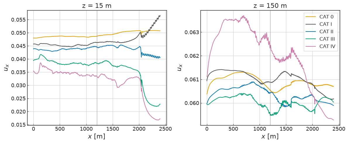
Mean velocity along the fetch at the 15 m and 150 m full-scale heights, for every category. The profiles should be statistically homogeneous well before the reference station at 1200 m.

def development_profile(sim_cfg: SimulationConfigs, line_name: str):
    """Time-mean ux along a streamwise probe line, vs x in metres."""
    df, points = read_line_series(sim_cfg, "development", line_name)
    x_m = points["x"].to_numpy(dtype=float) * M_PER_NODE
    u_mean = np.array([df[str(idx)].mean() for idx in points["idx"]], dtype=float)
    order = np.argsort(x_m)
    return x_m[order], u_mean[order]


fig, ax = common.fig_double()
for i, line_name in enumerate(["long_profile_15m", "long_profile_150m"]):
    for sim_name, (label, _, _) in CATEGORIES.items():
        x_m, u_mean = development_profile(sim_cfgs[sim_name, 0], line_name)
        ax[i].plot(x_m, u_mean, label=label)
    ax[i].axvline(1200.0, color=common.colors.refline, linewidth=1.0, alpha=0.7)
    ax[i].set_xlabel(r"$x$ [m]")
    ax[i].set_ylabel(r"$u_x$")
ax[0].set_title("z = 15 m")
ax[1].set_title("z = 150 m")
ax[1].legend()
plt.tight_layout()
plt.show(fig)

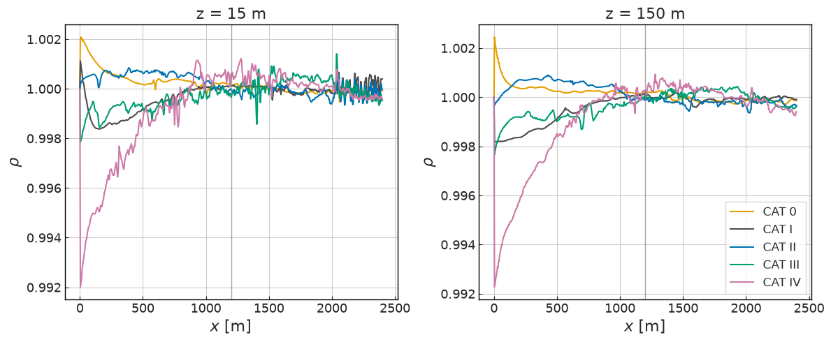
Streamwise development of density along the same probe lines. rho is not exported on the development lines (velocity only), so it is sampled from the instantaneous full-domain volume snapshot.

import pyvista as pv

from nassu import viz


def development_profile_rho(sim_cfg: SimulationConfigs, line_name: str):
    """Instantaneous rho along a streamwise probe line, vs x in metres.

    rho is not exported on the development probe lines (velocity only), so it is
    sampled from the last full-domain volume snapshot along the same line points.
    """
    line = sim_cfg.output.exports["development"].series.lines[line_name]
    points = pd.read_csv(line.points_filename).sort_values("x")
    x_m = points["x"].to_numpy(dtype=float) * M_PER_NODE
    xyz = points[["x", "y", "z"]].to_numpy(dtype=float)
    src = viz.FieldSource.from_cfg(sim_cfg, export="full_domain")
    vol = src.read(max(src.steps), derived=False)
    grid = vol.combine() if hasattr(vol, "n_blocks") else vol
    rho = np.asarray(pv.PolyData(xyz).sample(grid)["rho"], dtype=float)
    return x_m, rho


fig, ax = common.fig_double()
for i, line_name in enumerate(["long_profile_15m", "long_profile_150m"]):
    for sim_name, (label, _, _) in CATEGORIES.items():
        x_m, rho = development_profile_rho(sim_cfgs[sim_name, 0], line_name)
        ax[i].plot(x_m, rho, label=label)
    ax[i].axvline(1200.0, color=common.colors.refline, linewidth=1.0, alpha=0.7)
    ax[i].set_xlabel(r"$x$ [m]")
    ax[i].set_ylabel(r"$\rho$")
ax[0].set_title("z = 15 m")
ax[1].set_title("z = 150 m")
ax[1].legend()
plt.tight_layout()
plt.show(fig)

Flow field

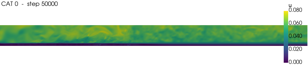
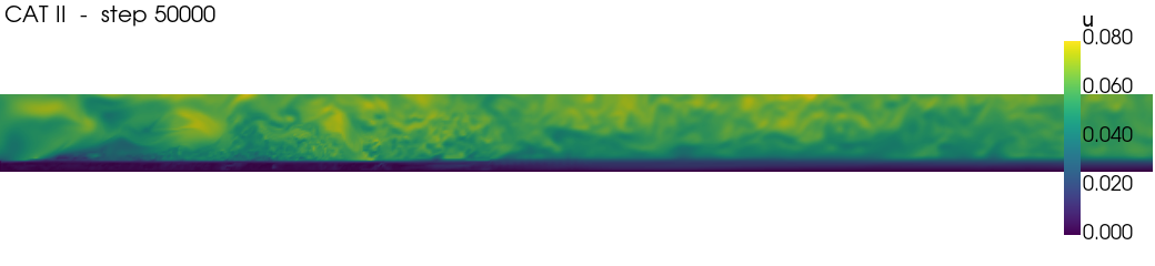
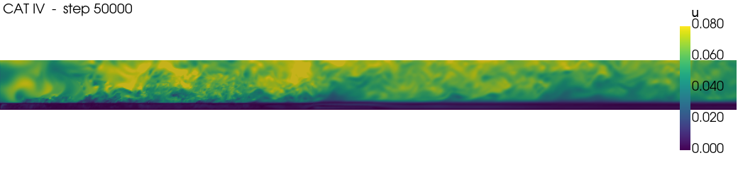
Instantaneous velocity magnitude on the coarse vertical mid-width plane (plane_series.mid_width, bounded to the boundary layer region), showing the turbulent boundary layer developing over the roughness fins.

viz.enable_offscreen()

PANEL = (1040, 240)
plane_pos = 80.0  # mid-width (lattice units)
FLOW_CATS = ("category_0_s4m", "category_2_s4m", "category_4_s4m")

view = viz.frame_domain((600.0, 160.0, 40.0), "y", panel=PANEL, slice_coord=plane_pos)

# Streamwise (x-z) mid-width plane coloured by velocity magnitude. One image per
# category - a single side-by-side grid of these very wide panels is unreadable.
for name in FLOW_CATS:
    source = viz.PlaneSource.from_cfg(sim_cfgs[name, 0], series="plane_series", plane="mid_width")
    panel = viz.Panel(CATEGORIES[name][0], source, view)
    plotter = viz.render_grid(
        [panel],
        steps=[max(source.steps)],
        scalar="u_mag",
        cmap="viridis",
        clim=(0.0, 0.08),
        bar_title="|u|",
        panel_size=PANEL,
    )
    plotter.show()

/tmp/ipykernel_1248290/146349723.py:25: UserWarning: Using static image for notebook display.
Install trame for interactive backends: pip install "pyvista[jupyter]"
  plotter.show()

Version

sim_cfg = sim_cfgs["category_4_s4m", 0]
sim_info = sim_cfg.output.read_info()

nassu_commit = sim_info["commit"]
nassu_version = sim_info["version"]
print("Version:", nassu_version)
print("Commit hash:", nassu_commit)

Version: 2.0.0a0
Commit hash: aaa6995a09d88707a467e1a8e1de7fc7f229de5b

Configuration

from IPython.display import Code

Code(filename=filename)

# Atmospheric boundary layer over five Eurocode 1 terrain categories
# (CAT 0-IV), aligned with the published validation study
# (https://docs.aerosim.io/validation/cases/vel_turb/abl.html) and the
# guided-case setup methodology
# (https://docs.aerosim.io/aerosim/guided-cases/ABL/setup.html).
#
# Scale 1/8: one level-0 lattice unit = 8 m full-scale; the refined slab
# around the measurement axis is 4 m. Reference height H = 150 m
# (18.75 lattice units), U_H = 0.06 -> Re_H = U_H * H / nu = 337,500.
#
# Reported quantities (notebook): mean velocity, turbulence intensity,
# integral length scales and energy spectra at the reference station,
# against the Eurocode 1 logarithmic profiles.

variables:
  simul:
    # Convective time scale CTS = H / U_H = 18.75 / 0.06 = 312.5 steps.
    # Statistics window: published T / CTS = 128 -> 40,000 steps, after a
    # 32 CTS development time.
    dev_time: 10000
    stats_time: 40000
    scale: !math 1/8
    plane_height: 5.01
    sigma_sem: 20
  domain:
    length: 600
    width: 160
    height: 112
  refine: &ANCHOR_VOLUMES_REFINE
    # Nested 3-level refinement wrapping the measurement axis (mirrors the
    # debug_DFSR ABL reference). Each level tightens around the station so the
    # near-ground ABL is resolved without a single wide coarse-fine interface
    # cutting the developing shear layer; the refinement starts just below the
    # IBM ground plane (z=2/3/4 < plane_height 5.01) and caps near 200 m.
    - start: [0.0, 65.0, 2.0]
      end: [250.0, 95.0, 25.0]
      lvl: 1
      is_abs: true
    - start: [0.0, 70.0, 3.0]
      end: [200.0, 90.0, 22.0]
      lvl: 2
      is_abs: true
    - start: [0.0, 73.0, 4.0]
      end: [170.0, 78.0, 10.0]
      lvl: 3
      is_abs: true
  var:
    # Reference station: 1200 m downstream of the inlet (canonical
    # measurement section of the published study).
    station_x: !math 1200 * ${simul.scale}
    # Probe heights above the IBM ground plane (full-scale metres * scale).
    z_15m: !math ${simul.plane_height} + (15 * ${simul.scale})
    z_150m: !math ${simul.plane_height} + (150 * ${simul.scale})
    # Profiles stop at 200 m full-scale - the validity limit of the
    # Eurocode 1 targets. Do not sample above this.
    z_200m: !math ${simul.plane_height} + (200 * ${simul.scale})
    # PODFS precursor plane extent. Unlike the Eurocode profiles above, the
    # precursor records the full inflow for replay, so it spans the whole ABL:
    # 200 m to each side of the spanwise centre and up to 400 m height.
    podfs_y_min: !math "0.5*${domain.width} - (200 * ${simul.scale})"
    podfs_y_max: !math "0.5*${domain.width} + (200 * ${simul.scale})"
    z_400m: !math "${simul.plane_height} + (400 * ${simul.scale})"

## Same variables to dependencies

simulations:
  - name: category_0_s4m
    save_path: ./validation/wind_engineering/01_atmospheric_boundary_layer/results/sem
    run_simul: true

    n_steps: !math "${simul.dev_time} + ${simul.stats_time}"

    report:
      frequency: 500
    checkpoint:
      export:
        interval: {frequency: 10000, start_step: !math "${simul.dev_time}"}
        finish_save: true
        keep_only_last_checkpoint: true

    data:
      monitors:
        fields:
          macrs_stats:
            macrs: [rho, u]
            stats: [min, max, mean]
            interval: {start_step: 0, frequency: 10}
      exports:
        full_domain:
          macrs: [rho, u]
          interval:
            frequency: 12500
            lvl: 0
          target:
            volume: {}
          outputs:
            instantaneous: true
        full_stats:
          macrs:
            - rho
            - u
          interval:
            frequency: 10
            start_step: !sub "${simul.dev_time}"
            lvl: 0
          target:
            volume: {}
          outputs:
            instantaneous: false
            stats:
              macrs_1st_order:
                - rho
                - u
              macrs_2nd_order:
                - u
        station:
          macrs: ["u"]
          interval: {frequency: 2, lvl: 0, start_step: !sub "${simul.dev_time}"}
          target:
            lines:
              reference_station:
                dist: 0.25
                start_pos: !math ["${var.station_x}", "0.5*${domain.width}", "${simul.plane_height}"]
                end_pos: !math ["${var.station_x}", "0.5*${domain.width}", "${var.z_200m}"]
          outputs:
            instantaneous: true
        development:
          macrs: ["u"]
          interval: {frequency: 50, lvl: 0, start_step: !sub "${simul.dev_time}"}
          target:
            lines:
              velocity_profile_010:
                dist: 0.25
                start_pos: !math [10, "0.5*${domain.width}", "${simul.plane_height}"]
                end_pos: !math [10, "0.5*${domain.width}", "${var.z_200m}"]
              velocity_profile_075:
                dist: 0.25
                start_pos: !math [75, "0.5*${domain.width}", "${simul.plane_height}"]
                end_pos: !math [75, "0.5*${domain.width}", "${var.z_200m}"]
              # Streamwise development at fixed full-scale heights.
              long_profile_15m:
                dist: 0.5
                start_pos: !math [0, "0.5*${domain.width}", "${var.z_15m}"]
                end_pos: !math [300, "0.5*${domain.width}", "${var.z_15m}"]
              long_profile_150m:
                dist: 0.5
                start_pos: !math [0, "0.5*${domain.width}", "${var.z_150m}"]
                end_pos: !math [300, "0.5*${domain.width}", "${var.z_150m}"]
          outputs:
            instantaneous: true
        plane_series:
          macrs: ["u"]
          interval: {frequency: 5000, lvl: 0}
          target:
            planes:
              # Coarse vertical streamwise overview plane at mid-width
              # (one node apart), bounded to the boundary layer region:
              # developing ABL over the roughness fins.
              mid_width:
                axis: y
                axis_pos: !math "0.5*${domain.width}"
                min: !math [0, 0]
                max: !math [600, 40]
                dist: 1
          # PODFS precursor recording. A dense, inlet-normal (YZ) plane at the
          # developed reference station: this is the precursor that the offline
          # `nassu podfs-build` compresses into a PODFS basis (POD in space +
          # Fourier series in time). The basis then replays as a `type: podfs`
          # inlet on a target case. SEM stays the default/interim inlet here -
          # this plane only records, it does not change the inflow.
          #
          # Sampled every 10 lvl-0 steps over the statistics window
          # (40,000 steps) -> ~4,000 snapshots, Fourier period T = 40,000 steps
          # (Nyquist period 20 steps). Lower the frequency to trade spectral
          # resolution for disk. Feed the resulting
          # `probes/precursor_inlet.planes.inlet_plane.xdmf` to a build-spec
          # `plane:` field (see 01_atmospheric_flow.podfs-build.yaml).
          outputs:
            instantaneous: true
        precursor_inlet:
          macrs: ["u"]
          interval: {frequency: 10, lvl: 0, start_step: !sub "${simul.dev_time}"}
          target:
            planes:
              # In-plane axes (y, z): 200 m to each side of the spanwise centre
              # (400 m span) and up to 400 m height, sampled at dist 0.25 lvl-0
              # nodes = 2 m full-scale -> a ~200 x 200 node analysis grid.
              inlet_plane:
                axis: x
                axis_pos: !math "${var.station_x}"
                min: !math ["${var.podfs_y_min}", "${simul.plane_height}"]
                max: !math ["${var.podfs_y_max}", "${var.z_400m}"]
                dist: 0.25

          outputs:
            instantaneous: true
    domain:
      domain_size:
        x: !sub "${domain.length}"
        y: !sub "${domain.width}"
        z: !math "${domain.height}"
      block_size: 8
      bodies:
        full_plane:
          IBM:
            order: 0
            cfg_use: plane_cfg
          geometry_path: fixture/stl/abl/ground.stl
          small_triangles: add
      global_transformations:
        - transformation:
            translation: !math [0, 0, "${simul.plane_height}"]
          point_clouds_apply: []
          bodies_apply: ["full_plane"]
          probes_apply: []
      refinement:
        static:
          lvl1:
            volumes_refine: *ANCHOR_VOLUMES_REFINE

    models:
      precision:
        default: single
      LBM:
        tau: 0.50001
        F:
          x: 0
          y: 0
          z: 0
        vel_set: D3Q27
        coll_oper: RRBGK
      initialization:
        inlet_field: true
      engine:
        name: CUDA
      BC:
        periodic_dims: [false, false, false]
        BC_map:
          - pos: E
            BC: RegularizedNeumannOutlet
            rho: 1.0
            wall_normal: E
            order: 2
          - pos: F
            BC: Neumann
            wall_normal: F
            order: 1
          - pos: B
            BC: RegularizedHWBB
            wall_normal: B
            order: 1
          - pos: N
            BC: Neumann
            wall_normal: N
            order: 0
          - pos: S
            BC: Neumann
            wall_normal: S
            order: 0
        inlet_turbulence:
          type: sem
          eddies:
            lengthscale: {x: !sub "${simul.sigma_sem}", y: !sub "${simul.sigma_sem}", z: !sub "${simul.sigma_sem}"}
            eddies_vol_density: 300
            domain_limits_yz:
              start: !math ["${simul.sigma_sem}", "-${simul.sigma_sem}"]
              end: !math ["${domain.width}-${simul.sigma_sem}", "${domain.height}-${simul.sigma_sem}"]
          profile:
            csv_profile_data: "./fixture/SEM/category_vprofile/profile_log_cat0_H150_Uh0.06.csv"
            z_offset: !math "${simul.plane_height}"
            length_mul: !math "${simul.scale}"

      LES:
        model: Smagorinsky
        sgs_cte: 0.17

      IBM:
        dirac_delta: 3_points
        forces_accomodate_time: 500
        body_cfgs:
          default:
            n_iterations: 3
            forces_factor: 1.0
          plane_cfg:
            n_iterations: 3
            forces_factor: 0.5
            wall_model:
              name: EqLog
              dist_ref: 3.125
              dist_shell: 0.125
              start_step: 300
              params:
                z0: !math "0.003*${simul.scale}"
                TDMA_max_error: 1e-04
                TDMA_max_iters: 10
                TDMA_min_div: 25
                TDMA_max_div: 25

      multiblock:
        overlap_F2C: 2

  - name: category_1_s4m
    parent: category_0_s4m
    run_simul: true

    domain:
      bodies:
        plates_obstacles:
          IBM:
            order: 1
          geometry_path: fixture/stl/abl/roughness_elements_cat1.stl
          volumes_limits:
            body_transformed:
              - start: !math [10, 20, 0]
                end: !math [300, "${domain.width} - 20", "0.5*${domain.height}"]
          small_triangles: add
          transformation:
            translation: [0, 1, 0]
            # abl/roughness_elements_cat*.stl are built at 1/10 scale (10 m
            # lattice) vs the old wind_tunnel plates' 1/32: factor 10/32.
            scale: !math ["20.0*${simul.scale}", "20.0*${simul.scale}", "10.0*${simul.scale}"] #1m
      global_transformations:
        - transformation: !not-inherit
            translation: !math [0, 0, "${simul.plane_height}"]
          point_clouds_apply: []
          bodies_apply: ["full_plane", "plates_obstacles"]
          probes_apply: []
    models:
      IBM:
        body_cfgs:
          plane_cfg:
            wall_model:
              params:
                z0: !math "0.01*${simul.scale}"
      BC:
        inlet_turbulence:
          type: sem
          profile:
            csv_profile_data: "./fixture/SEM/category_vprofile/profile_log_cat1_H150_Uh0.06.csv"

  - name: category_2_s4m
    parent: category_0_s4m
    run_simul: true

    domain:
      bodies:
        plates_obstacles:
          IBM:
            order: 1
          geometry_path: fixture/stl/abl/roughness_elements_cat2.stl
          volumes_limits:
            body_transformed:
              - start: !math [10, 20, 0]
                end: !math [300, "${domain.width} - 20", "${domain.height}"]
          small_triangles: add
          transformation:
            translation: [0, 1, 0]
            # abl/roughness_elements_cat*.stl are built at 1/10 scale (10 m
            # lattice) vs the old wind_tunnel plates' 1/32: factor 10/32.
            scale: !math ["20.0*${simul.scale}", "20.0*${simul.scale}", "10.0*${simul.scale}"] #2m
      global_transformations:
        - transformation: !not-inherit
            translation: !math [0, 0, "${simul.plane_height}"]
          point_clouds_apply: []
          bodies_apply: ["full_plane", "plates_obstacles"]
          probes_apply: []
    models:
      IBM:
        body_cfgs:
          plane_cfg:
            wall_model:
              params:
                z0: !math "0.05*${simul.scale}"
      BC:
        inlet_turbulence:
          type: sem
          profile:
            csv_profile_data: "./fixture/SEM/category_vprofile/profile_log_cat2_H150_Uh0.06.csv"

  - name: category_3_s4m
    parent: category_0_s4m
    run_simul: true

    domain:
      bodies:
        plates_obstacles:
          IBM:
            order: 1
          geometry_path: fixture/stl/abl/roughness_elements_cat2.stl
          volumes_limits:
            body_transformed:
              - start: !math [10, 20, 0]
                end: !math [300, "${domain.width} - 20", "${domain.height}"]
          small_triangles: add
          transformation:
            translation: [0, 1, 0]
            # abl/roughness_elements_cat*.stl are built at 1/10 scale (10 m
            # lattice) vs the old wind_tunnel plates' 1/32: factor 10/32.
            scale: !math ["20.0*${simul.scale}", "20.0*${simul.scale}", "3*10.0*${simul.scale}"] #6m
      global_transformations:
        - transformation: !not-inherit
            translation: !math [0, 0, "${simul.plane_height}"]
          point_clouds_apply: []
          bodies_apply: ["full_plane", "plates_obstacles"]
          probes_apply: []
    models:
      IBM:
        body_cfgs:
          plane_cfg:
            wall_model:
              params:
                z0: !math "0.3*${simul.scale}"
      BC:
        inlet_turbulence:
          type: sem
          profile:
            csv_profile_data: "./fixture/SEM/category_vprofile/profile_log_cat3_H150_Uh0.06.csv"

  - name: category_4_s4m
    parent: category_0_s4m
    run_simul: true

    domain:
      bodies:
        plates_obstacles:
          IBM:
            order: 1
          geometry_path: fixture/stl/abl/roughness_elements_cat2.stl
          volumes_limits:
            body_transformed:
              - start: !math [10, 20, 0]
                end: !math [300, "${domain.width} - 20", "${domain.height}"]
          small_triangles: add
          transformation:
            translation: [0, 1, 0]
            # abl/roughness_elements_cat*.stl are built at 1/10 scale (10 m
            # lattice) vs the old wind_tunnel plates' 1/32: factor 10/32.
            scale: !math ["20.0*${simul.scale}", "20.0*${simul.scale}", "5.0*10.0*${simul.scale}"] # 10m
      global_transformations:
        - transformation: !not-inherit
            translation: !math [0, 0, "${simul.plane_height}"]
          point_clouds_apply: []
          bodies_apply: ["full_plane", "plates_obstacles"]
          probes_apply: []
    models:
      IBM:
        body_cfgs:
          plane_cfg:
            wall_model:
              params:
                z0: !math "1.0*${simul.scale}"
      BC:
        inlet_turbulence:
          type: sem
          profile:
            csv_profile_data: "./fixture/SEM/category_vprofile/profile_log_cat4_H150_Uh0.06.csv"