Case 08: Buoyant channel - analytical validation of the Boussinesq coupling

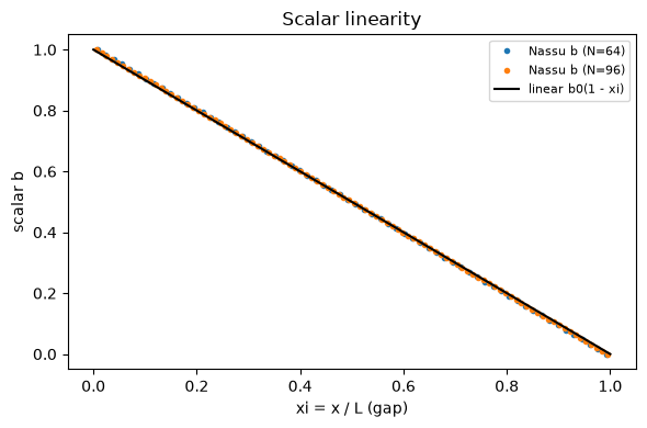
Laminar natural convection in a differentially-heated vertical channel isolates the Boussinesq body force F = rho0*beta*b*g (Guo source route): single block, no LES, no refinement, no IBM, no wall model - buoyancy is the only driver. A hot wall (phi = 1, low x) and a cold wall (phi = 0, high x) set an exactly linear scalar profile b(xi) = b0*(1 - xi); the buoyancy drives a steady vertical velocity w = uz with the closed form

\[w(\xi) = \frac{A}{12}\,(2\xi^3 - 3\xi^2 + \xi), \qquad A = \frac{\beta\,g_z\,b_0\,L^2}{\nu}, \qquad \xi = x/L,\]

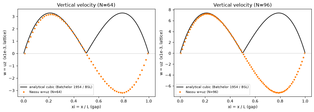
antisymmetric about the channel centre, with zeros at xi = 0, 1/2, 1, extrema at xi = 0.2113, 0.7887, and peak magnitude |A|/(72*sqrt(3)). Reference: the free-convection-between-vertical-plates solution (Batchelor 1954; Bird, Stewart & Lightfoot, Transport Phenomena).

Acceptance criterion (stated up front)

The exact solution is a continuum result; a finite-resolution LBM with halfway-bounce-back and regularized-Dirichlet walls carries a near-wall discretization error that is first order in the gap resolution. The case therefore validates on the shape and on convergence, not on a single tight number:

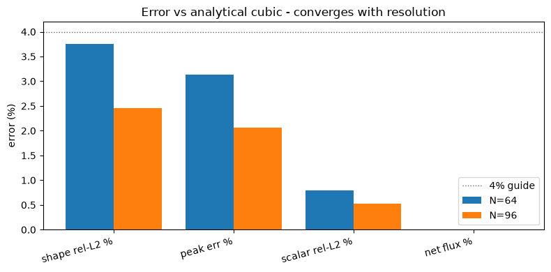
• antisymmetric cubic shape reproduced: profile relative-L2 vs the exact cubic < 4% at N=64, decreasing with resolution;

• peak location within +/-1 node of xi = 0.2113 / 0.7887 (exact);

• peak amplitude within 4% of |A|/(72*sqrt(3)) at N=64, decreasing with resolution (the convergence chart below must show the N=96 error below the N=64 error, confirming the residual is discretization);

• sign physical (hot / low-x side rises, c > 0);

• zero net flux |sum w| / (|w_peak|*N) < 1%;

• scalar linearity rel-L2 of b(xi) vs b0*(1 - xi) < 1% (input check).

Statistics (the late-window mean field), not instantaneous snapshots.

import glob
import pathlib

import h5py
import numpy as np
import matplotlib.pyplot as plt


def _find_project_root() -> pathlib.Path:
    here = pathlib.Path.cwd().resolve()
    for cand in [here, *here.parents]:
        if (cand / 'pyproject.toml').exists() and (cand / 'nassu').is_dir():
            return cand
    raise RuntimeError(f'Could not locate Nassu project root from {here}')


project_root = _find_project_root()
case = 'validation/wind_engineering/08_buoyant_channel'
results_dir = project_root / 'output' / case

# beta, g_z, b0, nu are fixed; only the gap L (= domain resolution) changes.
beta, g_z, b0, nu = 0.01, -1.0e-3, 1.0, 0.1
SIMS = {'N=64': ('buoyant_channel', 64), 'N=96': ('buoyant_channel_hires', 96)}
print('results dir:', results_dir, '(exists:', results_dir.exists(), ')')

results dir: /home/waine/Documents/Codigos/AeroSim/nassu-stratified-abl/output/validation/wind_engineering/08_buoyant_channel (exists: True )

Load mean fields and reduce to the wall-normal (gap) profile (guarded)

The gap axis is detected robustly as the axis carrying the scalar gradient (so the reduction is independent of the exported array’s axis order): the profile is the average of the time-mean field over the two homogeneous axes. w <- uz (the buoyancy-driven vertical component). Every loader returns None when the run is absent, so the plots degrade to ‘pending’.

def _gap_axis(field3):
    # the wall-normal (gap) axis is the one along which the scalar varies most
    ranges = []
    for ax in range(3):
        others = tuple(j for j in range(3) if j != ax)
        ranges.append(float(np.ptp(field3.mean(axis=others))))
    return int(np.argmax(ranges))


def load_profile(sim_name):
    pat = str(results_dir / f'{sim_name}__000' / 'outputs'
              / 'mean_fields.volume.mean_fields.stats.*.h5')
    files = sorted(glob.glob(pat))
    if not files:
        return None
    with h5py.File(files[-1], 'r') as h:
        blk = h[sorted(h.keys())[-1]]['block0']
        phi = np.asarray(blk['temperature_phi'][:])
        uz = np.asarray(blk['uz'][:])
    gax = _gap_axis(phi)
    others = tuple(j for j in range(3) if j != gax)
    w = uz.mean(axis=others)
    b = phi.mean(axis=others)
    N = w.size
    xi = (np.arange(N) + 0.5) / N
    return {'xi': xi, 'w': w, 'b': b, 'N': N}


def analytic(xi, Lgap):
    A = beta * g_z * b0 * Lgap**2 / nu
    return (A / 12.0) * (2 * xi**3 - 3 * xi**2 + xi), A


runs = {tag: load_profile(name) for tag, (name, _) in SIMS.items()}
have = {tag: r is not None for tag, r in runs.items()}
print('results present:', have)

results present: {'N=64': True, 'N=96': True}

Velocity profile vs the analytical cubic

The simulated w(xi) = uz at each resolution overlaid on the exact closed-form cubic. If the coupling is correct the markers sit on the curve and approach it as resolution increases.

fig, axes = plt.subplots(1, len(SIMS), figsize=(11, 4))
for ax, (tag, (name, Lgap)) in zip(np.atleast_1d(axes), SIMS.items()):
    r = runs[tag]
    if r is not None:
        xi = r['xi']
        xf = np.linspace(0, 1, 200)
        wex, A = analytic(xf, Lgap)
        g = 2 * xi**3 - 3 * xi**2 + xi
        c = float((r['w'] * g).sum() / (g * g).sum())  # match the code's sign
        ax.plot(xf, np.sign(c) * np.abs(wex) * 1e3, 'k-',
                label='analytical cubic (Batchelor 1954 / BSL)')
        ax.plot(xi, r['w'] * 1e3, 'C1o', ms=3, label=f'Nassu w=uz ({tag})')
    else:
        ax.text(0.5, 0.5, 'pending GPU run', ha='center', va='center', transform=ax.transAxes)
    ax.axhline(0, color='0.8', lw=0.8)
    ax.set_xlabel('xi = x / L (gap)')
    ax.set_ylabel('w = uz  (x1e-3, lattice)')
    ax.set_title(f'Vertical velocity ({tag})')
    if ax.get_legend_handles_labels()[0]:
        ax.legend(fontsize=8)
fig.tight_layout()
plt.show()

Scalar profile (input check)

The transported buoyancy scalar must be exactly linear across the gap; any deviation is the error in the buoyancy input and bounds the momentum match.

fig, ax = plt.subplots(figsize=(6, 4))
for tag, (name, Lgap) in SIMS.items():
    r = runs[tag]
    if r is not None:
        ax.plot(r['xi'], r['b'], 'o', ms=3, label=f'Nassu b ({tag})')
if any(have.values()):
    xf = np.linspace(0, 1, 50)
    ax.plot(xf, b0 * (1 - xf), 'k-', label='linear b0(1 - xi)')
    ax.legend(fontsize=8)
else:
    ax.text(0.5, 0.5, 'pending GPU run', ha='center', va='center', transform=ax.transAxes)
ax.set_xlabel('xi = x / L (gap)'); ax.set_ylabel('scalar b'); ax.set_title('Scalar linearity')
fig.tight_layout(); plt.show()

Convergence of the error with resolution

The acceptance metrics at each resolution as a grouped bar chart. The bars must decrease from N=64 to N=96 - the discretization error converging toward the analytical solution - which is what certifies the buoyancy coupling as correct rather than merely close at one grid.

def metrics(r, Lgap):
    xi = r['xi']; g = 2*xi**3 - 3*xi**2 + xi
    _, A = analytic(xi, Lgap); wmax = abs(A) / (72 * np.sqrt(3))
    c = float((r['w'] * g).sum() / (g * g).sum())
    shape = float(np.linalg.norm(r['w'] - c * g) / np.linalg.norm(c * g)) * 100
    peak = abs(abs(r['w']).max() - wmax) / wmax * 100
    scal = float(np.linalg.norm(r['b'] - b0 * (1 - xi)) / np.linalg.norm(b0 * (1 - xi))) * 100
    flux = abs(r['w'].sum()) / (abs(r['w']).max() * r['N']) * 100
    return {'shape rel-L2 %': shape, 'peak err %': peak, 'scalar rel-L2 %': scal,
            'net flux %': flux, 'sign hot-up': c > 0}

labels = ['shape rel-L2 %', 'peak err %', 'scalar rel-L2 %', 'net flux %']
fig, ax = plt.subplots(figsize=(8, 4))
tags = [t for t in SIMS if runs[t] is not None]
if tags:
    x = np.arange(len(labels)); w = 0.8 / len(tags)
    rows = {}
    for k, tag in enumerate(tags):
        m = metrics(runs[tag], SIMS[tag][1]); rows[tag] = m
        ax.bar(x + (k - (len(tags)-1)/2) * w, [m[l] for l in labels], w, label=tag)
    ax.axhline(4.0, ls=':', color='0.4', lw=1, label='4% guide')
    ax.set_xticks(x); ax.set_xticklabels(labels, rotation=15, ha='right')
    ax.set_ylabel('error (%)'); ax.legend()
    print('metric summary (supplement to the chart above):')
    for tag in tags:
        print(f'  {tag}: ' + ', '.join(f'{l}={rows[tag][l]:.3f}' for l in labels)
              + f", sign hot-up={rows[tag]['sign hot-up']}")
else:
    ax.text(0.5, 0.5, 'pending GPU run', ha='center', va='center', transform=ax.transAxes)
ax.set_title('Error vs analytical cubic - converges with resolution')
fig.tight_layout(); plt.show()

metric summary (supplement to the chart above):
  N=64: shape rel-L2 %=3.751, peak err %=3.139, scalar rel-L2 %=0.794, net flux %=0.001, sign hot-up=True
  N=96: shape rel-L2 %=2.462, peak err %=2.069, scalar rel-L2 %=0.525, net flux %=0.005, sign hot-up=True

Verdict

The case passes when, at both resolutions, the simulated w(xi) reproduces the antisymmetric analytical cubic (peak location exact, physical sign, zero net flux, linear scalar) and the shape / peak error decreases from N=64 to N=96 - the discretization error converging toward the exact solution. A monotone drop certifies the Boussinesq buoyancy coupling; a static or growing error would flag a coupling defect. This is the analytical, single-block, feature-alone rung the composition matrix rests on.